Next: Gradients and Directional Derivatives
Up: Lecture_12_web
Previous: Scalar Functions with Vector Argument
Next: Gradients and Directional Derivatives
Up: Lecture_12_web
Previous: Scalar Functions with Vector Argument
Subsections
There is no doubt that a great deal confusion arises from the
following question, ``What are the variables of my function?''
For example, suppose we have a three-dimensional space  ,
in which there is an embedded surface
,
in which there is an embedded surface
 =
=
 where
where
 is a
vector that lies in the surface,
and an embedded curve
is a
vector that lies in the surface,
and an embedded curve
 .
Furthermore, suppose there is a curve that lies within the surface
.
Furthermore, suppose there is a curve that lies within the surface
 .
.
Suppose that
 is a scalar function of
.
is a scalar function of
.
Here are some questions that arise in different applications:
- How does
 vary as a function of position?
- How does
vary along the surface?
- How does
vary along the curve?
- How does
vary along the curve embedded in the surface?
Taylor Series
The behavior of a function near a point is something that arises frequently
in physical models.
When the function has lower-order continuous partial derivatives (generally,
a ``smooth'' function near the point in question), the stock method to
model local behavior is Taylor's series expansions around a fixed point.
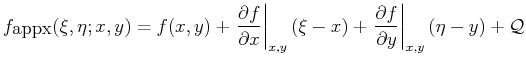
Taylor's expansion for a scalar function of  variables,
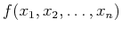 which has continuous first and second partial
derivatives near the point
which has continuous first and second partial
derivatives near the point
 is:
is:
![\begin{displaymath}\begin{split}& f(\xi_1 , \xi_2 , \ldots , \xi_n) = f(x_1 , x_...
...] +\ldots + \mathcal{O}\left[(\xi_n - x_n)^3\right] \end{split}\end{displaymath}](img54.png) |
(12-8) |
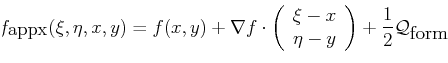
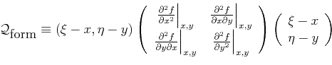
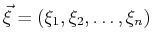
or in a vector shorthand:
![$\displaystyle f(\vec{x}) = f(\vec{\xi}) + \left.\nabla_{\vec{x}} f\right\vert _...
...dot (\vec{xi} - \vec{x}) +\mathcal{O}\left[\norm {\vec{\xi} - \vec{x}}^3\right]$](img55.png) |
(12-9) |
MATHEMATICA Example
 |
| (notebook Lecture-12) |
| (html Lecture-12) |
| (xml+mathml Lecture-12) |
Approximating Surfaces
Example of turning a function of two variables,  into
an approximating function of four variables:
into
an approximating function of four variables:
- Start with a function
and expand it about a point
 to second order--use
MATHEMATICA
's Normal function to convert from
series representation to a parabolic representation.
to second order--use
MATHEMATICA
's Normal function to convert from
series representation to a parabolic representation.
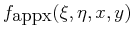
- The expansion is now a function of four variables--the first two variables
are the point the function is expanded around, and the second two are the
variable of the parabolic approximation at that point:
where
or
where
- Plot the function
 for
for
 and
and
 for a selected number of points
  .
.
|
Just a few of many examples of instances where Taylor's expansions are used are:
- linearization
- Examining the behavior of a model near a point
where the model is understood.
Even if the model is wildly non-linear, a useful approximation is
to make it linear by evaluating near a fixed point.
- approximation
- If a model has a complicated representation in terms
of unfamiliar functions, a Taylor expansion can be used to characterize
the `local' model in terms of a simple polynomials.
- asymptotics
- Even when a system has singular behavior (e.g, the
value of a function becomes infinite as some variable approaches a
particular value), how the system becomes singular is very important.
At singular points, the Taylor expansion will have leading order terms that are
singular, for example near
 ,
,
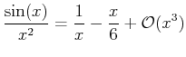 |
(12-10) |
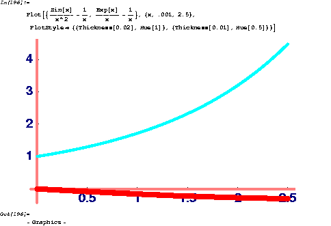
The singularity can be subtracted off and it can be said that this
function approaches  "linearly" from below with slope -1/6.
Comparing this to the behavior of another function that is singular
near zero:
"linearly" from below with slope -1/6.
Comparing this to the behavior of another function that is singular
near zero:
 |
(12-11) |
shows that the  behavior is ``more singular.''
Figure 12-1:
Behavior of two singular functions near their
singular points.

|
- stability
- In the expansion of energy about a point
is obtained, then the various orders of expansion can be interpreted:
- zero-order
- The zeroth-order term in a local expansion is
the energy of the system at the point evaluated.
Unless this term is to be compared to another point, it
has no particular meaning (if it is not infinite) as
energy is always arbitrarily defined up to a constant.
- first-order
- The first-order is related to the driving force
to change the state of the system. Consider:
 |
(12-12) |
If force exists, the system can decrease it energy linearly by picking
a particular change
 that is anti-parallel to the
force.
that is anti-parallel to the
force.
For a system to be stable, it is a necessary first condition that
the forces (or first order expansion coefficients) vanish.
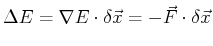
- second order
- If a system has no forces on it (therefore
satisfying the necessary condition of stability), then where
the system is stable or unstable depends on whether a
small
can be found that deceases the energy:
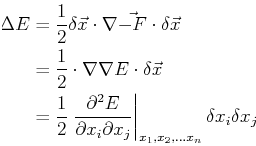 |
(12-13) |
where the summation convention is used above and the point
 is one for which
  is zero.
- numerics
- Derivatives are often obtained numerically in
numerical simulations.
The Taylor expansion provides a formula to approximate numerical
derivatives--and provides an estimate of the numerical error
as a function of quantities like numerical mesh size.
© W. Craig Carter 2003-, Massachusetts Institute of Technology