Solution Free Energies that Generate Phase Diagrams

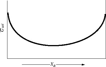
For the construction of phase diagrams, plausible forms of the free energy of solution have been utilized without discussion of their derivation. For instance,

Figure 31-6: Prototype of the Molar Gibbs Free Energy of Solution.

Previously, the ideal solution was defined for the case where the chemical potential of each component is a linear function of the log of its mole fraction:

$$\input{equations/mu-IS}$$ (31-1)

which implies that:

$$\input{equations/G-IS}$$ (31-2)

which does give the qualitative features that are drawn in Figure 31-6.

One might wonder why such a simple form of the molar Gibbs free energy of solution would be used for condensed phases, since this is the form that was derived from ideal gases.

One condition of equilibrium is that the chemical potential in each phase must be equal. Therefore if the vapor phase above a condensed phase is in equilibrium then:

$$\mu^{sol}_i = \mu^{vap}_i$$

Considering an ideal gas as the vapor (another assumption):

$$\input{equations/23-2A}$$ (31-3)

The second term it is what we derived for the ideal solution:

$$\input{equations/23-2B}$$ (31-4)

where $\gamma^{IS}$ is independent of $X_i$.