Last Time

Growth of Precipitates (After Nucleation

Coarsening

Coarsening: Mean Field Theories and Particle Size Distributions

Gibbs-Thompson Effect

Grain Growth

3.21 Spring 2002: Lecture 22

Continuous Transformations--Introduction

In previous lectures on morphological evolution by surface diffusion, interface motion arises even though there is no transportation of material through the interface.

For the case of evaporation-condensation, interface motion arises because material is transforming from a state on one side of the interface into the state on the other side of the interface.

Evaporation-condensation is a simple example of a kinetic process associated with a phase transformation: interface velocity is related to the rate (volume/time) of phase transformation per unit area of interface. Discussions of phase transformations are facilitated with a definition of phase The concept of a phase is often confused with heterogeneity. It will become apparent that a system with multiple phases is necessarily heterogeneous and necessarily has interfaces However, the converse--a heterogeneous system with interfaces necessarily has multiple phases--is not true and is easily proved by the existence of polycrystalline single phase material or that of antiphase boundaries.

Phase

A homogeneous part of a system that can be identified as ``physically different'' from another part of the system. Physically different implies that the two homogeneous subsystems are not related by a combined rotation and translation. A phase is always separated from another phase by an identifiable interface.

Pedestrian examples are the solid phases, liquid phase, and vapor phase of pure water where the homogeneous phase can be identified by homogeneous values of the mass density or enthalpy density--the interface can be identified by those regions where the field parameters representing densities of equilibrium extensive quantities are spatially variable. Less obvious examples are the FCC and BCC phases of iron-carbon-nickel-chromium steel or the ferromagnetic and non-ferromagnetic phases of LaSrMnO manganites.

I'll take this opportunity to quote one of my heros:

We may call such bodies as differ in composition or state, different phases of the matter considered, regarding all bodies which differ only in quantity and form as different examples of the same phase.

&dotfill#dotfill;J. W. GIBBS in Trans. Connecticut Acad. III. (1875) page 152

Figure: A single component phase diagram. On the right figure, the color represents the equilibrium value of a molar extensive quantities (i.e., blue is a low value of $\ensuremath{\overline{V}}$ and red is a large value of $\ensuremath{\overline{V}}$) that apply to each phase at that particular $p$ and $T$. For phase transitions, the color could be associated with an order parameter.

The motion of a grain boundary or an antiphase domain boundary does not transform material as it passes through it. The material is re-ordered but not transformed. Nevertheless, it is useful to introduce a field parameter characterizing the local symmetry or spatial orientation of a material. Such a field parameter would have the characteristic of being uniform except in the vicinity of grain boundary or antiphase domain boundary.

In either case, the kinetic evolution of the relevant field parameter becomes a convenient means to track the motion of the interface because the interface can be co-located at values of the field parameter intermediate to its homogeneous values in the abutting material.

Such field parameters are generically called order parameters. Although it may be that ``order parameter'' has a natural conceptual association to the case of geometrical variants of a single phase, it is consistent with the use of order parameters in the Landau expansion of a free energy density about its equilibrium density. We shall use order parameters in either case.

The hypothesis that an order parameter changes continously through an interface is connected to questions of whether a phase change or geometrical change can be continuous transformations. In other words, a phase or geometrical variant can be generated within another by a continuous process.

The process of the formation of a new phase from an existing phase can be classified into two categories: continuous and discontinuous phase transitions.

Discontinuous phase transitions occur by nucleation--a process that Gibbs called, ``... initially small in extent but great in degree.''¹

Degree refers to quantity that characterized a phase and extent refers a length scale. Nucleation will be treated in subsequent lectures.

Continuous phase transitions can be treated with the evolution of continuous order parameter fields--processes that Gibbs called, ``initially is small in degree, but may be great in its extent in space.''

Considerations of the development of a continuous phase transformations or geometrical transform should begin with a careful examination of order parameters.

Order Parameters

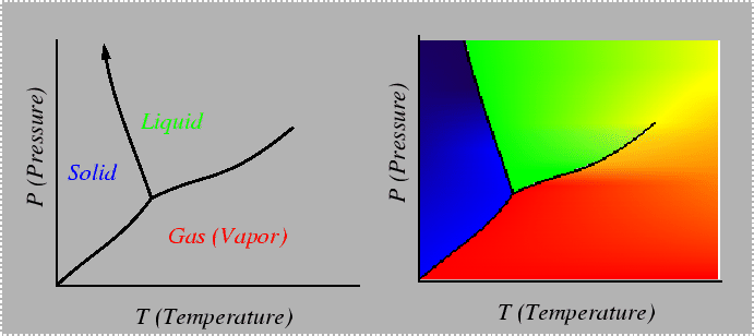
Consider a system in which composition cannot be varied, such as a pure material. The Gibbs phase rule indicates that there is only one degree of freedom in a system that can characterized by temperature and pressure only. One degree of freedom implies that for conditions in which two phases are in equilibrium, there must be a relation between temperature and pressure. Such a relation can be derived by considering the Gibbs-Duhem relationship in each of the phases--for example, if the two phases are solid and liquid:

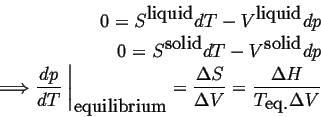$$\begin{split}0 = \ensuremath{{S}^{\mbox{liquid}}}dT - \ensure... ...\Delta V} = \frac{\Delta H}{T_{\mbox{eq.}}\Delta V} \end{split}$$ (22-1)

which is the famous Clausius-Clapeyron equation that couples changes in intensive parameters so that phase equilibrium is continuously satisfied.

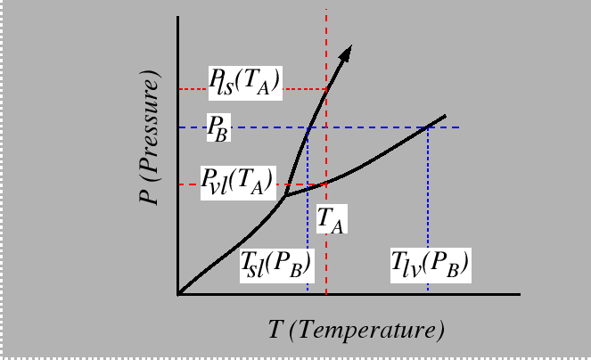
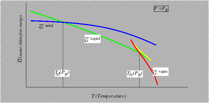
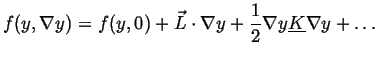
Consider the behavior of the molar free energy (or $\mu$) on slices of Figure 22-1 at constant $p$ and $T$:

Figure 22-2: Considerations of the molar Gibbs free energy on slices of the single component phase diagram along lines of constant $T$ and constant $p$. The slope of the curve is related to the molar volume of each phase and can be used as an order parameter that indicates the spatial variation of a phase.

Figure: Behavior of $\ensuremath{\overline{G}} = \mu$ at constant $P$ as a function of $T$. Where the curvature of $\ensuremath{\overline{G}}$ changes sign, the system is unstable to small fluctuations in density. The liquid and vapor curves must be connected to each other and this is illustrated with the "spiny-looking" curve with opposite curvature. The solid curve is not continuously connected to the others.

Figure: Behavior of $\ensuremath{\overline{G}} = \mu$ at constant $T$ as a function of $p$. The slope of the curve is related to the molar volume of each phase and can be used as an order parameter that indicates the spatial variation of a phase.

Figure 22-5: Example of single component phase diagram plotted with one derived intensive variable.

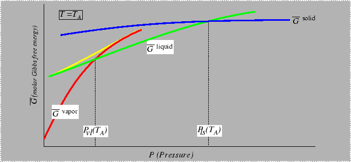What would the plot look like with two extensive variables plotted?

The example in 22-5 is reminiscent of a phase diagram with a miscibility gap:

Figure 22-6: Illustration of the types of free energy curves and the regions on a phase diagram that are associated with spinodal decomposition.

In fact, if one of the chemical potentials that can be derived by the graphical tangent intercept method was plotted as a function of composition, it would look very similar to the "spiny-looking" curves in Figs 22-3 and 22-3.

In the case of a phase transformation, the equilibrium values of the density of an extensive quantity, such as the concentration or composition $c(\vec{x})$, can be used as an order parameter. For geometric transformations or order-disorder, a similar approach of equilibrium hidden variables is implicit in a Landau expansion.².

Consider two phases that differ by an order parameter $\eta$ that could be associated with the displacement of an atom away from a crystalline inversion center, such as in a piezoelectric transition. The equilibrium state of the crystal as an arbitrary function of a fixed temperature and pressure can be approximated as a series in the terms $p$, $T$, and $\eta$:

$$\ensuremath{\overline{G}}(T,p,\eta) = \ensuremath{\overline{G_o}}(T,p) + a(p) (T - T_c) \eta^2 + B(p) \eta^4$$ (22-2)

where $T_c$ is the Curie temperature for the transition. The equilibrium state of is entirely determined by the minima of $\ensuremath{\overline{G}}$ as a function of pressure and temperature--therefore $\eta$ does not have have the same status as the variables $T$ and $p$. The order parameter $\eta$ is determined by the minima of $\ensuremath{\overline{G}}$:

$$\eta_{equil}^2 = \frac{a(P) (T - T_c)}{2 B(p)}$$ (22-3)

In the case of phase transformations above, the molar volume could be used as a local indicator of which phase is present--$\ensuremath{\overline{V}}(\vec{x})$ can be used as an order parameter field. Similarly, spatial variations of a field $\eta(\vec{x})$ could be used as an order parameter to indicate whether a phase is in its centrosymmetric or a piezoelectric phase--and positions where $\vert\ensuremath{\nabla}\eta\vert$ is large would identify interfaces.

Because a common description language can be developed, it is useful to consider the similarities between different kinds of order parameters; i.e, the densities of extensive quantities that are used as order parameters for phase transformations and the geometrical (or hidden) variables that serve as order parameters that can be used to identify an interface in a single phase material. However, differences between the two types of order parameters will have important consequences on the kinetics of their evolution.

An important distinction is that one order parameter (e.g., $c(\vec{x})$) is locally conserved--local changes can only arise from a flux divergence in the absence of sources and sinks. The other type of order parameter is not locally conserve; e.g., a measure of disorder $\eta(\vec{x})$ can change with no associated flux.

Figure 22-7: Illustration of two atomic rearrangement processes.

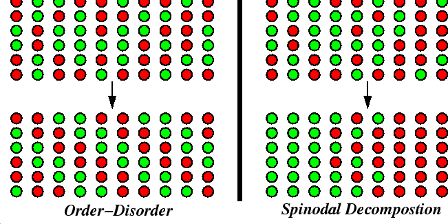The ordering reaction does not require long-range diffusion, but the decomposition reaction must move mass over long distances.

In the appendix to these notes, it is demonstrated how the changes in free energy depend on whether flux is required or not. The important results can be summarized as follows:

• Non-conserved quantities: If $\eta$ is a non-conserved quantity, like spin, or crystalline order, then for small changes in $\eta$ given by $\delta \eta$:

  $$\Delta {G} = \delta \eta \frac{d {G}}{d\eta} \ensuremath{\left.\mbox{\rule{0pt}{16pt}}\right\vert}_{\eta = \eta_0}$$ (22-4)

  
  

  Therefore, an order parameter can always decrease the free energy by picking a variation $\delta \eta$ with a sign that makes the product in Eq. 22-23 negative. An non-conserved order parameter has no barrier against reaching a value which makes the free energy a local minimum.

  
  

• Conserved quantities: If $c$ is a non-conserved quantity, like concentration, then for small changes in $c$ given by $\delta c$:

  $$\Delta {G} = \frac{1}{2} (\delta c)^2 \frac{d^2 {G}}{dc^2} \ensuremath{\left.\mbox{\rule{0pt}{16pt}}\right\vert}_{c = c_0}$$ (22-5)

  
  

  Therefore, a barrier to the growth of small variations exists whenever the second derivative in Eq. 22-22 is positive. Thus, nucleation is required for a transformation outside of the spinodal curves.

  In fact, it can be shown that the sign of the diffusivity, $D$, for concentration flux is given by the second derivative ${\partial^2 {G}}/{\partial c^2}$. This has the effect of causing ``up-hill'' diffusion.

  
  

Kinetics and Diffuse Interfaces

If transformations occur without nucleation, then the thermodynamics must account for continuous variations of thermodynamic state variables. These continuous variations are called ``diffuse interfaces'' and they are addressed in this section. The important result is that the local free energy density has a contribution due to gradients of thermodynamic state variables.

The theory for the free energy of inhomogeneous systems was developed by Cahn and Hilliard in 1958. The theory was originally developed to account for contributions to the free energy from gradients in the composition--or any other conserved field. The diffuse interface method was extended to non-conserved order parameters by Allen and Cahn (1979) in their study of the kinetics of the order-disorder transition. The theories for both can be developed in parallel since their construction follows from the same principles. $c(\vec{x})$ describes any conserved field quantity (like the concentration field in a closed system) and $\eta(\vec{x})$ represents any non-conserved order parameter field.

A two-phase system with a miscibility gap at equilibrium with a planar interface will have an equilibrium composition profile $c(x)$ through the interfacial region. The form of the equilibrium composition distribution is determined by the $c(x)$ which minimizes $F$, the total free energy of the system. Similarly, a system that tends to form long-range ordered domains will have a distribution of order, $\eta(x)$, across a planar interface between two identical domains having different local minima in their order parameters.

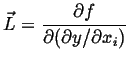
Example profiles, $c(x)$ and $\eta(x)$, through diffuse interfaces in these two types of systems are shown schematically below:

Figure 22-8: Illustration of order parameter fields in the diffuse interface theories.

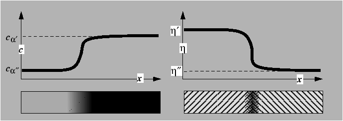The profiles $c(x)$ and $\eta(x)$ are continuous and the compositions $c_{\alpha'}$ and $c_{\alpha''}$ are the equilibrium compositions of the bulk phases. The values of order parameter $\eta'$ and $\eta''$ correspond to local minima in the free energy.

Let $y(x)$ stand for either $c(x)$ or $\eta(x)$. Also, let $f(y,\nabla y)$ be the free energy of a small volume $dV$ which has average composition $y$ and a gradient $\nabla y$ across it. If the free energy density is expanded about its homogeneous value $f(y) = f(y,0)$ (presumably a known function) then then

$$f(y, \nabla y) = f(y,0) + \vec{L} \cdot \nabla y + \frac{1}{2} \nabla y \underline{K} \nabla y + \ldots$$ (22-6)

where

$$\vec{L} = \frac{\partial f}{\partial (\partial y /\partial x_i)}$$ (22-7)

is a vector evaluated at zero gradient and

$$\underline{K} = \frac{\partial^2 f}{ \partial (\partial y /\partial x_i) \partial (\partial y /\partial x_j) }$$ (22-8)

is a matrix of second derivatives.

If homogeneous material has a center of symmetry, the free energy cannot depend on the direction of the gradient and thus $\vec{L} = 0$ and $\underline{K}$ will be a symmetric matrix. Furthermore, if the homogeneous material is isotropic (or cubic), then $\underline{K}$ will be a diagonal matrix (with components $K$ along the diagonal), then free energy density is, to second order:

$$f(y, \nabla y) = f(y,0) + \frac{K}{2} \nabla y \cdot \nabla y = f(y,0) + \frac{K}{2} \vert\nabla y\vert^2$$ (22-9)

Only the second term contributes to the free energy only in the region near the interface (where the gradient is non-zero). The gradient-energy coefficient $K$ is a parameter which contributes to the interfacial area. However, it is not the only term which contributes: as the composition profile traverses the interface region, compositions from the non-equilibrium parts of the free energy curve are contributing to the excess free energy associated with the interface as well.

It is possible to calculate equilibrium profiles in terms of the parameters in Eq. 22-9. However, our purpose is describe the kinetics of how an arbitrary distribution $y(\vec{x})$ evolves towards equilibrium.

We will take a variational calculus approach. The treatment below assumes no prior knowledge of the calculus of variations and will serve as an introduction to the subject.

The total free energy of the entire system (occupying the domain $\Omega$) is:

$$F[y(x)] = \int_\Omega ( f(y) + \frac{K}{2} \nabla y \cdot \nabla y) dV$$ (22-10)

which defines $F$ as a functional with the argument $y(\vec{x})$³. The function $y(\vec{x})$ will also have specified boundary conditions on $\partial \Omega$ (the boundary of $\Omega$); for instance, $y(\partial \Omega)$ will have fixed values or fixed derivatives.

If the field $y(\vec{x})$ is changing with velocity $v(\vec{x})$, the is the rate of change of $F$ is

$$F(y + vt) = \int_\Omega [ f(y+ vt) + + \frac{K}{2} ( \nabla y \cdot \nabla y + 2 t \nabla y \cdot \nabla v + t^2 \nabla v \cdot \nabla v ] dV$$ (22-11)

so that

$$\frac{\partial F}{\partial t} \ensuremath{\left.\mbox{\rule{0pt}{16pt}}\right\vert}_{t=0} = \int_\Omega [ f'(y) v + K \nabla y \cdot \nabla v ] dV$$ (22-12)

using

$$\nabla \cdot(v \nabla y) = \nabla v \cdot \nabla y + v \nabla^2 y$$ (22-13)

and using the divergence theorem,

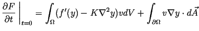$$\frac{\partial F}{\partial t} \ensuremath{\left.\mbox{\rule{0pt}{... ... f'(y) - K \nabla^2 y ) v dV + \int_{\partial \Omega} v \nabla y \cdot d\vec{A}$$ (22-14)

The boundary integral vanishes if $v(\partial \Omega) = 0$, which would be the case if $y(\partial \Omega)$ had fixed boundary values⁴; or, if the projections of the gradients onto the boundary vanish. If these two cases are not satisfied, then when the volume to surface ratio is greater than the inherent diffusion length, the system may be considered to be large enough so that the contributions due to boundary can be neglected.

The change in total energy in Eq. 22-14 is the sum of local variations: $( f'(y) - K \nabla^2 y ) v$. Therefore, the largest possible increase of $F$ is when the flow, $v(\vec{x})$, is proportional to

$$f'(y) - K \nabla^2 y$$ (22-15)

Therefore, Equation 22-15 is the functional gradient of $F(y)$.⁵Sometimes Eq. 22-15 is called the variational derivative of $F$.⁶When the variational derivative vanishes, $y(x)$ is an extremal function and a candidate for a local maximum or minimum. For the case of the gradient energy, if Eq. 22-15 vanishes, then $y$ is an equilibrium profile.

The functional gradient is the starting point for the kinetic equations for conserved and non-conserved parameter fields.

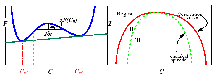
Appendix: Free Energy Changes and Geometric Constructions

The free energy versus composition curve, illustrated in the above for a constant temperature, is a familiar example of a free energy which gives rise to a miscibility gap. The region between the spinodal lines delimits those compositions for which there is no barrier to decomposition. Inside the miscibility gaps, but outside of the spinodal region, decomposition is favored but a thermodynamic barrier requires large fluctuations in composition (i.e., nucleation) for decomposition. The position of spinodal lines is determined by the sign of the free energy change for a small fluctuation in composition. The following derivation is from Hilliard which derives the variation of the molar free energy, $\overline{F}(c)$, but this derivation applies to any extensive molar quantity.⁷.

We can write $\overline{F}(c)$ in terms of its partial molar quantities, $\overline{F}_A(c)$ and $\overline{F}_B(c)$:

$$\begin{array}{ll} \overline{F}(c) & = \frac{N_A}{N_A + N_B} \... ... c) \overline{F}_B(c) = c \mu_A(c) + (1-c) \mu_B(c) \end{array}$$ (22-16)

which plots as a straight line when the arguments of the partial molar quantities are evaluated at a particular point $c_0$ on the curve $\overline{F}(c)$: $c \mu_A(c_0) + (1-c) \mu_B(c_0)$. Consider a large system at composition $c_0$ which transforms 1 mole to a new composition $c'$. If the system is open and the composition is free to change, then the change in $\overline{F}$ is simply the difference $\Delta \overline{F} = \overline{F}(c') - \overline{F}(c_0)$. Similarly, for any non-conserved parameter $\eta$, the change in molar free energy is:

$$\Delta \overline{F} = \overline{F}(\eta') - \overline{F}(\eta)$$ (22-17)

Figure 22-9: Illustration of the change in molar free energy from a composition $c_0$. If the system is closed so the composition is fixed, then the change in the molar free energy is $\Delta \overline{F}_c$ for every mole which forms at composition $c'$. If the system is open and the composition is free to change its value, then $\Delta \overline{F}_u$ is the change per mole transformed.

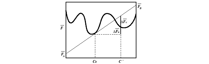However, if the system is closed (which is the case for a localized fluctuation in composition), then it is necessary to account for the exchange of material necessary to satisfy the constraint of fixed composition. For each mole transformed, the change in $\overline{F}$ for the $c'$ moles of the $B$ component is $[ \overline{F}_B(c') - \overline{F}_B(c_0)]c'$, with a similar term for the $A$ component:

$$\Delta \overline{F} = [ \overline{F}_B(c') - \overline{F}_B(c_0)]c' + [ \overline{F}_A(c') - \overline{F}_A(c_0)](1 - c')$$ (22-18)

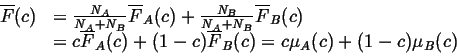
which can be rewritten as

$$\begin{array}{ll} \Delta \overline{F} = & c' \overline{F}_B(c... ... - c') [ \overline{F}_B(c_0) - \overline{F}_A(c_0)] \end{array}$$ (22-19)

or

$$\Delta \overline{F} = \overline{F}(c') - \overline{F}(c_0) - (c' ... ...verline{F}}{dc} \ensuremath{\left.\mbox{\rule{0pt}{16pt}}\right\vert}_{c = c_0}$$ (22-20)

which is numerically equal to the distance indicated in the figure by the distance $\Delta \overline{F}_c$. $\Delta \overline{F}_c$ is negative if the curve for $\overline{F}(c)$ lies below the tangent at $c = c'$. Equation 22-20 holds for any concentration $c'$ when the composition $c_0$ is fixed.

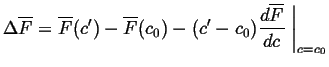
Consider the special case of a small composition fluctuation, $\delta c = c' - c_0$. Expanding $\overline{F}(c)$ in $\delta c$:

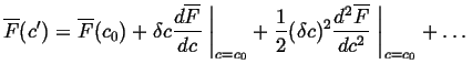$$\overline{F}(c') = \overline{F}(c_0) + \delta c \frac{d \overline... ...{dc^2} \ensuremath{\left.\mbox{\rule{0pt}{16pt}}\right\vert}_{c = c_0} + \ldots$$ (22-21)

Substituting Eq. 22-20 into Eq. 22-21 results in the change in the molar free energy for a variation of a conserved parameter $c$:

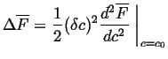$$\Delta \overline{F} = \frac{1}{2} (\delta c)^2 \frac{d^2 \overline{F}}{dc^2} \ensuremath{\left.\mbox{\rule{0pt}{16pt}}\right\vert}_{c = c_0}$$ (22-22)

Similarly, the lowest order term for the change in the molar free energy for a variation of a non-conserved order parameter $\eta$ is

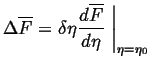$$\Delta \overline{F} = \delta \eta \frac{d \overline{F}}{d\eta} \ensuremath{\left.\mbox{\rule{0pt}{16pt}}\right\vert}_{\eta = \eta_0}$$ (22-23)

Therefore, an order parameter can always decrease the free energy by picking a variation $\delta \eta$ with a sign that makes the product in Eq. 22-23 negative. An non-conserved order parameter has no barrier against reaching a value which makes the free energy a local minimum.

On the other hand, for a conserved quantity like $c$, the variation in molar free energy is proportional to $(\delta c)^2$. Therefore, a barrier to the growth of small variations exists whenever the second derivative in Eq. 22-22 is positive. Thus, nucleation is required for a transformation outside of the spinodal curves.

The sign of Eq. 22-22 determines the sign of the interdiffusion coefficient.

• About this document ...