For the two-dimensional linear system
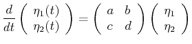 |
(25-5) |
Every two-by-two matrix has two invariants (i.e., values that do not depend on a unitary
transformation of coordinates).
These invariants are the trace, ![]() of the matrix (the sum of all the diagonals) and
the determinant
of the matrix (the sum of all the diagonals) and
the determinant ![]() .
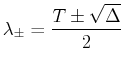
The eigenvalue equation can be written in terms of these two invariants:
.
The eigenvalue equation can be written in terms of these two invariants:
| (25-6) |
 |
(25-7) |
The curves separating these regions have singular behavior.
For example, where ![]() for positive
for positive ![]() , the eigenvalues are purely
imaginary and trajectories circulate about the fixed point in a stable
orbit.
This is called a center and
is the case for an undamped harmonic oscillator.
, the eigenvalues are purely
imaginary and trajectories circulate about the fixed point in a stable
orbit.
This is called a center and
is the case for an undamped harmonic oscillator.
The regions can be mapped with the invariants and the following diagram illustrates the behavior.

At the point where the five regions come together, all the entries of the matrix of coefficients are zero and the physical behavior is then determined by expanding Eq. 25-1 to the next highest order at which the coefficients are not all zero.
|
MATHEMATICA |
| (notebook Lecture-25) |
| (html Lecture-25) |
| (xml+mathml Lecture-25) |
| Predicting Behavior at a Fixed Point in the Plane
|
|
MATHEMATICA |
| (notebook Lecture-25) |
| (html Lecture-25) |
| (xml+mathml Lecture-25) |
| Visualizing the Behavior at a Fixed Point in the Plane
|
The phase portraits that were visualized in the above example help illustrate a very powerful mathematical method from non-linear mechanics.
Consider the saddle-node that has one positive (unstable) and one negative (stable) eigenvalue. Those initial points that are located in regions where the negative (stable) eigenvalue dominates are quickly swept towards the fixed point and then follow the unstable direction away from the fixed point. Roughly speaking, the stable values are `smashed' onto the unstable direction and virtually all of the motion takes place near the unstable direction.
This idea allows a large system (i.e., one in which
the vector
![]() has many components) to
be reduced to a smaller system in which the stable directions have been approximated
by a thin region near the trajectories associated with the unstable eigenvalues.
This is sometimes called reduction of ``fast variables'' onto the unstable manifolds.
has many components) to
be reduced to a smaller system in which the stable directions have been approximated
by a thin region near the trajectories associated with the unstable eigenvalues.
This is sometimes called reduction of ``fast variables'' onto the unstable manifolds.