Link to Current (updated) notes

Phase Plane and Critical Points

A few examples of physical models that can be represented by systems of first-order differential equations:

$$\ensuremath{\frac{d{\vec{y}}}{d{t}}} \equiv \ensuremath{\frac{d{}... ...c{y},t)\ \vdots\ F_N(\vec{y},t) \end{array} \right) \equiv \vec{F}(\vec{y},t)$$ (25-1)

and, furthermore, it has been shown that many higher-order systems of ODEs can be reduced to larger systems of first-order ODEs.

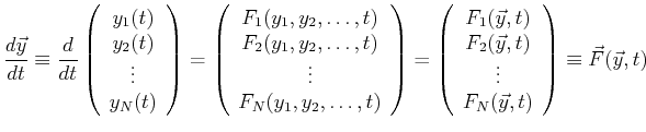
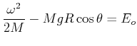
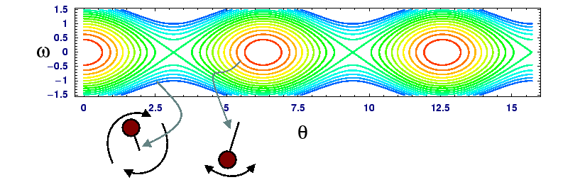
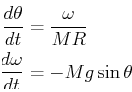
The behavior of systems of first-order equations can be visually interpreted by plotting the trajectories $\vec{y}(t)$ for a variety of initial conditions $\vec{y}(t=0)$ . An illustrative example is provided by the equation for the pendulum, $M R^2 \ddot{\theta} + M g R \sin \theta = 0$ . can be re-written with the angular momentum $\omega$ as the system of first-order ODEs

$$\begin{split}\ensuremath{\frac{d{\theta}}{d{t}}} & = \frac{\o... ...remath{\frac{d{\omega}}{d{t}}} & = -M g \sin \theta \end{split}$$ (25-2)

which was shown in Lecture 22 to have solutions:

$$\frac{\omega^2}{2 M} - M g R \cos \theta = E_o$$ (25-3)

Eq. 25-3 can be used to plot the the trajectories in the phase plane.

Figure: Example of the phase plane for the pendulum equation. The small closed orbits are the stable harmonic oscillations about the stable position $\stackrel{\vert}{\bullet}$ . The larger orbits are those with increasing energy until the energy is just large enough that the pendulum rises to its unstable equilibrium position $\stackrel{\bullet}{\vert}$ . The two kinds of fixed points (i.e., the stable and unstable points where $\dot{\omega} = \dot{\theta} = 0$ ) regulate the portrait of the phase plane. (Note: The word ``phase'' here should not be confused with the common usage of phase in materials science. In the current context for example, the phase represents the positions and momenta of all the particles in a system--this usage is important in statistical mechanics. However, the word ``phase'' in materials science and engineering is usually interpreted as a portion of material that lies within an identifiable interface--this usage is implied in ``equilibrium phase diagrams.'')

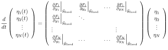
Behavior for a wide variety of initial conditions can be comprehended by the following approach:

Identify Fixed Points

If all the points in the phase plane where $d\vec{y}/dt = 0$ can be established, then these fixed points can be used as reference points around which the phase-behavior will be determined.

Linearization

At each fixed point, Linearization is obtained by expanding Eq. 25-1 to first order in $\vec{\eta} = \vec{y} - \vec{y}_{\text{fixed}}$ , the zeroth-order term vanishes by construction:

$$\ensuremath{\frac{d{}}{d{t}}}\left( \begin{array}{c} \eta_1(t)\ ... ...) \left( \begin{array}{c} \eta_1\ \eta_2\ \vdots\ \eta_N \end{array} \right)$$ (25-4)

Eigenvalues/Eigenvectors

When the system Eq. 25-4 is transformed into a coordinate frame in which the matrix is diagonal, then each component of $\vec{\eta}_{\text{eigen-frame}}$ has a trajectory that is unaffected by the others and determined by only the diagonal entry associated with that component.

The $\vec{\eta}_{\text{eigen-frame}}$ are the eigenvectors of Eq. 25-4 and the diagonal component is its associated eigenvalue.

Fixed Point Characterization

If the eigenvalue is real, then any point that lies in the direction of its eigenvector will evolve along a straight path parallel to the eigenvector. If the real eigenvalue is negative, that straight path will asymptotically approach the origin; if the eigenvalue is positive the trajectory will diverge along the straight-path towards infinity.

If the eigenvalue is imaginary, then the trajectory will circulate about the fixed point with a frequency proportional the eigenvalue's magnitude.

If the eigenvalue, $\lambda$ is complex, its trajectory will both circulate with a frequency proportional to its imaginary part and diverge from or converge to the fixed point according to $\eta_o \exp($Re${\lambda})$ .

If any one of the fixed points has an eigenvalue with a positive real part, the fixed point cannot be stable--this is because ``typical'' points in the neighborhood of the fixed points will possess some component of the unstable eigenvector.