
 Next: Index
Up: Lecture_22_web
Previous: Differential Operators
Next: Index
Up: Lecture_22_web
Previous: Differential Operators
Subsections
Methods for finding general solution to the linear inhomogeneous
second-order ODE
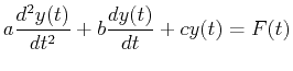 |
(22-21) |
have been developed and worked out in
MATHEMATICA examples.
Eq. 22-21 arises frequently in physical models,
among the most common are:
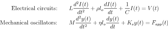 |
(22-22) |
where:
| |
Mechanical |
Electrical |
Second
Order |
Mass  :
Physical measure of the ratio of
momentum field to velocity
:
Physical measure of the ratio of
momentum field to velocity |
Inductance  :
Physical measure of the ratio of stored
magnetic field to current
:
Physical measure of the ratio of stored
magnetic field to current |
First
Order |
Drag Coefficient

( is viscosity
 is a unit displacement):
Physical measure of the ratio environmental resisting
forces to velocity--or proportionality constant
for energy dissipation with square of velocity
is a unit displacement):
Physical measure of the ratio environmental resisting
forces to velocity--or proportionality constant
for energy dissipation with square of velocity |
Resistance

( is resistance per unit
material length
is resistance per unit
material length
 is a unit length):
Physical measure of the ratio of voltage drop
to current--or proportionality constant for power
dissipated with square of the current.
is a unit length):
Physical measure of the ratio of voltage drop
to current--or proportionality constant for power
dissipated with square of the current. |
Zeroth
Order |
Spring Constant  :
Physical measure of the ratio environmental force
developed to displacement--or proportionality constant
for energy stored with square of displacement
:
Physical measure of the ratio environmental force
developed to displacement--or proportionality constant
for energy stored with square of displacement |
Inverse Capacitance  :
Physical measure of the ratio of voltage storage rate
to current--or proportionality constant for energy storage rate
dissipated with square of the current.
:
Physical measure of the ratio of voltage storage rate
to current--or proportionality constant for energy storage rate
dissipated with square of the current. |
Forcing
Term |
Applied Voltage  :
Voltage applied to circuit as a function of time.
:
Voltage applied to circuit as a function of time. |
Applied Force  :
Force applied to oscillator as a function of time.
:
Force applied to oscillator as a function of time. |
For the homogeneous equations (i.e. no applied forces
or voltages) the solutions for physically allowable values
of the
coefficients can either be oscillatory, oscillatory
with damped amplitudes, or, completely damped with no oscillations.
(See Figure ![[*]](crossref.png) ).
The homogeneous equations are sometimes called autonomous
equations--or autonomous systems.
).
The homogeneous equations are sometimes called autonomous
equations--or autonomous systems.
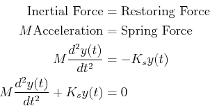
The simplest version of a homogeneous
Eq. 22-21 with no damping coefficient ( ,
,  , or
, or  )
appears in a remarkably wide variety of physical models.
This simplest physical model is a simple harmonic oscillator--composed
of a mass accelerating with a linear spring restoring force:
)
appears in a remarkably wide variety of physical models.
This simplest physical model is a simple harmonic oscillator--composed
of a mass accelerating with a linear spring restoring force:
 |
(22-23) |
Here  is the displacement from the equilibrium position-i.e., the
position where the force,
is the displacement from the equilibrium position-i.e., the
position where the force,
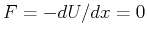 .
Eq. 22-23 has solutions that oscillate in time with frequency
.
Eq. 22-23 has solutions that oscillate in time with frequency  :
:
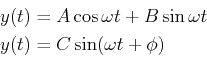 |
(22-24) |
where
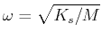 is the natural frequency of oscillation,
 and
and  are integration constants written as amplitudes; or,
  and
and  are integration constants written as an amplitude and a phase shift.
The simple harmonic oscillator has an invariant, for the
case of mass-spring system the invariant is the total energy:
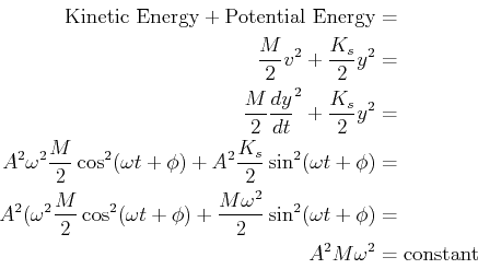 |
(22-25) |
There are a remarkable number of physical systems that can be reduced to
a simple harmonic oscillator (i.e., the model can be reduced to
Eq. 22-23).
Each such system has an analog to a mass, to a spring constant, and thus
to a natural frequency.
Furthermore, every such system will have an invariant that is an analog
to the total energy--an in many cases
the invariant will, in fact, be the total energy.
The advantage of reducing a physical model to a harmonic oscillator is
that all of the physics follows from the simple harmonic oscillator.
Here are a few examples of systems that can be reduced to simple harmonic
oscillators:
- Pendulum
- By equating the rate of change of angular momentum equal to the
torque, the equation for pendulum motion can be derived:
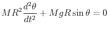 |
(22-26) |
for small-amplitude pendulum oscillations,
 ,
the equation is the same as a simple harmonic oscillator.
,
the equation is the same as a simple harmonic oscillator.
It is instructive to consider the invariant for the non-linear equation.
Because
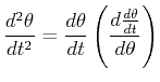 |
(22-27) |
Eq. 22-26 can be written as:
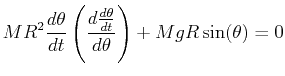 |
(22-28) |
![$\displaystyle \ensuremath{\frac{d{}}{d{\theta}}}\left[\frac{M R^2}{2} \left( \ensuremath{\frac{d{\theta}}{d{t}}} \right)^2 - Mg R \cos(\theta)\right] = 0$](img106.png) |
(22-29) |
which can be integrated with respect to  :
:
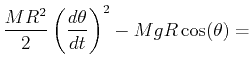 constant constant |
(22-30) |
This equation will be used as a level-set equation to visualize pendulum
motion.
- Buoyant Object
- Consider a buoyant object that is slightly displaced from its
equilibrium floating position.
The force (downwards) due to gravity of the buoy is
 The force (upwards) according to Archimedes is
 where
where  is the volume of the buoy that is submerged.
The equilibrium position must satisfy
is the volume of the buoy that is submerged.
The equilibrium position must satisfy
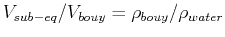 .
.
If the buoy is slightly perturbed at equilibrium by an amount  the force is:
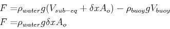 |
(22-31) |
where  is the cross-sectional area at the equilibrium position.
Newton's equation of motion for the buoy is:
is the cross-sectional area at the equilibrium position.
Newton's equation of motion for the buoy is:
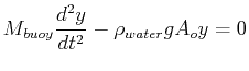 |
(22-32) |
so the characteristic frequency of the buoy is
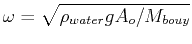 .
.
- Single Electron Wave-function
- The one-dimensional Schrödinger equation is:
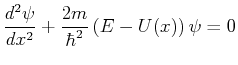 |
(22-33) |
where  is the potential energy at a position
  .
If
.
If
 is constant as in a free electron in a box, then
the one-dimensional wave equation reduces to a simple
harmonic oscillator.
is constant as in a free electron in a box, then
the one-dimensional wave equation reduces to a simple
harmonic oscillator.
In summation, just about any system that oscillates about
an equilibrium state can be reduced to a harmonic oscillator.
© W. Craig Carter 2003-, Massachusetts Institute of Technology