Next: Harmonic Oscillators
Up: Lecture_22_web
Previous: Lecture_22_web
Next: Harmonic Oscillators
Up: Lecture_22_web
Previous: Lecture_22_web
Subsections
The idea of a function as ``something'' that takes a value
(real, complex, vector, etc.) as ``input'' and returns ``something else''
as ``output'' should be very familiar and useful.
This idea can be generalized to operators
that take a function as an argument and return
another function.
The derivative operator operates on a function
and returns another function that describes how
the function changes:
![\begin{displaymath}\begin{split}\mathcal{D}[f(x)] & = \ensuremath{\frac{d{f}}{d{...
...)]\\ \mathcal{D}[f(x) + g(x)] = & D[f(x)] + D[g(x)] \end{split}\end{displaymath}](img1.png) |
(22-1) |
The last two equations above indicate
that the ``differential operator'' is a linear operator.
The integration operator is the right-inverse of

![$\displaystyle \mathcal{D} [\mathcal{I}[ f(x)]] = \mathcal{D}[ \int f(x) dx]$](img3.png) |
(22-2) |
but is only the left-inverse up to an arbitrary constant.
Consider the differential operator that returns a constant
multiplied by itself
 |
(22-3) |
which is another way to write the
the homogenous linear first-order ODE and
has the same form as an eigenvalue equation.
In fact,
 , can be
considered an eigenfunction of
Eq. 22-3.
, can be
considered an eigenfunction of
Eq. 22-3.
For the homogeneous second-order equation,
![$\displaystyle \left(\mathcal{D}^2 + \beta \mathcal{D} - \gamma \right)[ f(x)] = 0$](img6.png) |
(22-4) |
It was determined that there were two eigensolutions that can
be used to span the entire solution space:
 |
(22-5) |
Operators can be used algebraically,
consider the inhomogeneous second-order ODE
![$\displaystyle \left(a \mathcal{D}^2 + b \mathcal{D} + c\right)[y(x)] = x^3$](img8.png) |
(22-6) |
By treating the operator as an algebraic quantity, a
solution can be found1
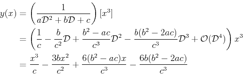 |
(22-7) |
which solves Eq. 22-6.
The Fourier transform is also a linear operator:
![\begin{displaymath}\begin{split}\mathcal{F}[f(x)] =& g(k) = \frac{1}{\sqrt{2 \pi...
...i}} \int_{-\infty}^{\infty} g(k) e^{-\imath k x} dk \end{split}\end{displaymath}](img10.png) |
(22-8) |
Combining operators is another useful way to solve differential equations.
Consider the Fourier transform,
 , operating on the
differential operator,
, operating on the
differential operator,
 :
:
![$\displaystyle \mathcal{F}[\mathcal{D}[f]] = \frac{1}{\sqrt{2 \pi}} \int_{-\infty}^{\infty} \ensuremath{\frac{d{f(x)}}{d{x}}} e^{i k x} dx$](img13.png) |
(22-9) |
Integrating by parts,
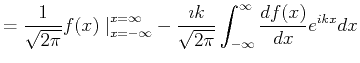 |
(22-10) |
If the Fourier transform of  exists, then typically2
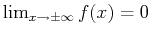 .
In this case,
.
In this case,
![$\displaystyle \mathcal{F}[\mathcal{D}[f]] = -i k \mathcal{F}[f(x)]$](img19.png) |
(22-11) |
and by extrapolation:
![\begin{displaymath}\begin{split}\mathcal{F}[\mathcal{D}^2[f]] & = -k^2 \mathcal{...
...{D}^n[f]] & = (-1)^n \imath^n k^n \mathcal{F}[f(x)] \end{split}\end{displaymath}](img20.png) |
(22-12) |
Consider the heterogeneous second-order linear ODE which
represent a forced, damped, harmonic oscillator that
will be discussed later in this lecture.
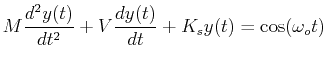 |
(22-13) |
Apply a Fourier transform (mapping from the time ( ) domain to
a frequency (
) domain to
a frequency ( ) domain) to both sides of 22-13:
![\begin{displaymath}\begin{split}\mathcal{F}[M \ensuremath{\frac{d^2{y(t)}}{d{t}^...
...ta(\omega-\omega_o) +\delta(\omega+\omega_o)\right] \end{split}\end{displaymath}](img24.png) |
(22-14) |
because the Dirac Delta functions result from taking the
Fourier transform of
 .
.
Equation 22-14 can be solved for the Fourier
transform:
![$\displaystyle \mathcal{F}[y] = \sqrt{\frac{-\pi}{2}} \frac{ \left[ \delta(\omeg...
...ega_o) +\delta(\omega+\omega_o)\right] } { M \omega^2 + \imath \omega V - K_s }$](img26.png) |
(22-15) |
In other words, the particular solution Eq. 22-13
can be obtained by finding the
function  that has a Fourier transform equal the
the right-hand-side of Eq. 22-15-or, equivalently,
operating with the inverse Fourier transform on the
right-hand-side of Eq. 22-15.
that has a Fourier transform equal the
the right-hand-side of Eq. 22-15-or, equivalently,
operating with the inverse Fourier transform on the
right-hand-side of Eq. 22-15.
MATHEMATICA Example
 |
| (notebook Lecture-22) |
| (html Lecture-22) |
| (xml+mathml Lecture-22) |
| Operator Calculus and the Solution to the Damped-Forces Harmonic
Oscillator Model
MATHEMATICA does have built-in functions to take Fourier (and other kinds of)
integral transforms.
However, as will be seen below, using operational calculus to
solve ODEs is not necessarily simple in
MATHEMATICA
does have built-in functions to take Fourier (and other kinds of)
integral transforms.
However, as will be seen below, using operational calculus to
solve ODEs is not necessarily simple in
MATHEMATICA .
Nevertheless, it may be instructive to force it--if only as an
an example of using the good tool for the wrong purpose.
.
Nevertheless, it may be instructive to force it--if only as an
an example of using the good tool for the wrong purpose.
|
Operators to Functionals
Equally powerful is the concept of a functional which
takes a function as an argument and returns a value.
For example
![$ \mathcal{S}[y(x)]$](img31.png) , defined below, operates on
a function
, defined below, operates on
a function  and returns its surface of revolution's area
for
and returns its surface of revolution's area
for  :
:
![$\displaystyle \mathcal{S}[y(x)] = 2 \pi \int_0^L y \sqrt{1 + \left(\ensuremath{\frac{d{y}}{d{x}}}\right)^2} dx$](img34.png) |
(22-16) |
This is the functional to be minimized for the question, ``Of all
surfaces of revolution that span from  to
to  ,
which is the
,
which is the  that has the smallest surface area?''
This idea of finding ``which function maximizes or minimizes something''
can be very powerful and practical.
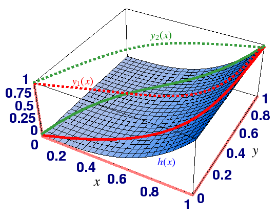
Suppose you are asked to run an ``up-hill'' race from some starting
point  to some ending point
  and there
is a ridge
and there
is a ridge
 .
What is the most efficient running route
.
What is the most efficient running route  ?3
?3
Figure:
The terrain separating the
starting point
 and ending point
 .
Assuming a model for how much running speed slows with the
steepness of the path--which route would be quicker, one (
.
Assuming a model for how much running speed slows with the
steepness of the path--which route would be quicker, one ( )
that starts going up-hill at first or another (
)
that starts going up-hill at first or another ( ) that initially
traverses a lot of ground quickly?
) that initially
traverses a lot of ground quickly?

|
A reasonable model for running speed as a function of climbing-angle  is
is
 |
(22-17) |
where  is the arclength along the path.
The maximum speed occurs on flat ground
is the arclength along the path.
The maximum speed occurs on flat ground  and running
speed monotonically falls to zero as
and running
speed monotonically falls to zero as
 .
To calculate the time required to traverse any path
.
To calculate the time required to traverse any path  with endpoints
 and
and  ,
,
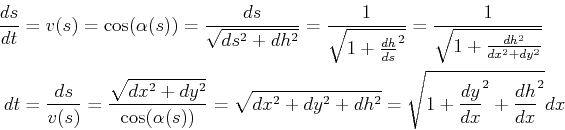 |
(22-18) |
So, with the hill  , the time as a functional of the
path is:
, the time as a functional of the
path is:
![$\displaystyle \mathcal{T}[y(x)] = \int_0^1 \sqrt{1 + {\ensuremath{\frac{d{y}}{d{x}}}}^2 + 4 x^2} \; dx$](img61.png) |
(22-19) |
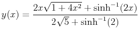
There is a powerful and beautiful mathematical method for
finding the extremal functions of functionals which is
called Calculus of Variations.
By using the calculus of variations, the optimal path  for
Eq. 22-19 can be determined:
for
Eq. 22-19 can be determined:
 |
(22-20) |
The approximation determined in the
MATHEMATICA example above is
pretty good.
example above is
pretty good.
© W. Craig Carter 2003-, Massachusetts Institute of Technology