Link to Current (updated) notes

Second Order ODEs with Constant Coefficients

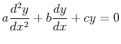
The most simple case--but one that results from models of many physical phenomena--is that functions in the homogeneous second-order linear ODE (Eq. 21-5) are constants:

$$a \ensuremath{\frac{d^2{y}}{d{x}^2}} + b \ensuremath{\frac{d{y}}{d{x}}} + c y = 0$$ (21-9)

If two independent solutions can be obtained, then any solution can be formed from this basis pair.

Surmising solutions seems a sensible strategy, certainly for shrewd solution seekers. Suppose the solution is of the form $y(x) = \exp(\lambda x)$ and put it into Eq. 21-9:

$$(a \lambda^2 + b \lambda + c) e^{\lambda x} = 0$$ (21-10)

which has solutions when and only when the quadratic equation $a \lambda^2 + \lambda x + c = 0$ has solutions for $\lambda$ .

Because two solutions are needed and because the quadratic equation yields two solutions:

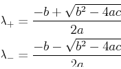
$$\begin{split}\lambda_+ &= \frac{-b + \sqrt{b^2 - 4 a c}}{2 a}\ \lambda_- &= \frac{-b - \sqrt{b^2 - 4 a c}}{2 a} \end{split}$$ (21-11)

or by removing the redundant coefficient by diving through by $a$ :

$$\begin{split}\lambda_+ &= \frac{-\beta}{2} + \sqrt{(\frac{\be... ...c{-\beta}{2} - \sqrt{(\frac{\beta}{2})^2 - \gamma } \end{split}$$ (21-12)

where $\beta \equiv b/a$ and $\gamma \equiv c/a$ .

Therefore, any solution to Eq. 21-9 can be written as

$$y(x) = C_+ e^{\lambda_+ x} + C_- e^{\lambda_- x}$$ (21-13)

MATHEMATICA$^{\text{\scriptsize {\textregistered }}}$ Example

(notebook Lecture-21)

(html Lecture-21)

(xml+mathml Lecture-21)

Solutions to $\ensuremath{\frac{d^2{y}}{d{x}^2}} + \beta \ensuremath{\frac{d{y}}{d{x}}} + \gamma y = 0$

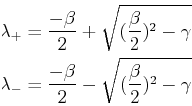
Because the fundamental solution depend on only two parameters $\beta$ and $\gamma$ , the behavior of all solutions can be visualized in the $\gamma$ -$\beta$ plane.

1. Insert $y(x) = \exp(\lambda x)$ into the ODE $y'' + \beta y' + \gamma y = 0$ and solve for a condition on $\lambda$ that solutions exist (assuming real coefficients $\gamma$ and $\beta$ ).
2. Plot the condition that the roots are complex in the $\gamma$ -$\beta$ plane. This is the region of parameter space that gives oscillatory solutions (because $\exp(r + \imath \theta) = \exp(r)(\cos(x) + \imath \sin(x))$ )
3. Plot the conditions that the $\lambda$ are real--these are the monotonically growing ( $\lambda > 0$ ) or shrinking ( $\lambda < 0$ ) solutions
4. Plot the conditions that the real part is negative, this is the damped oscillatory region.
5. Plot the conditions that the real part is positive, this is the unbounded growth region.
6. Use the MATHEMATICA$^{\text{\scriptsize {\textregistered }}}$ function Reduce to find the three regions: $(\lambda_+ > 0 , \lambda_- > 0)$ --monotonically growing solutions, $(\lambda_+ > 0 , \lambda_- < 0)$ --one growing and one decaying solution, $(\lambda_+ < 0 , \lambda_- < 0)$ --monotonically decaying solutions.

The behavior of all solutions can be collected into a simple picture:

Figure 21-1: The behaviors of the linear homogeneous second-order ordinary differential equation $\ensuremath{\frac{d^2{y}}{d{x}^2}} + \beta \ensuremath{\frac{d{y}}{d{x}}} + \gamma y = 0$ plotted according the behavior of the solutions for all $\beta$ and $\gamma$ .

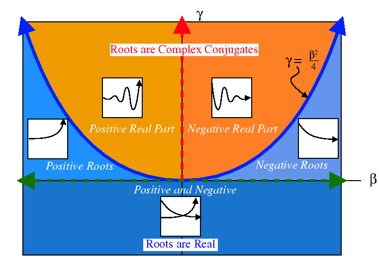
The case that separates the complex solutions from the real solutions, $\gamma = (\beta/2)^2$ must be treated separately, for the case $\gamma = (\beta/2)^2$ it can be shown that $y(x) = \exp(\beta x/2)$ and $y(x) = x \exp(\beta x/2)$ form an independent basis pair (see Kreyszig AEM, p. 74).