Link to Current (updated) notes

Higher-Order Equations: Background

For first-order ordinary differential equations (ODEs), $F(y'(x),y(x),x)$ , one value $y(x_o)$ was needed to specify a particular solution. For second-order equations, two independent values are needed. This is illustrated in the following forward-differencing example.

MATHEMATICA$^{\text{\scriptsize {\textregistered }}}$ Example

(notebook Lecture-21)

(html Lecture-21)

(xml+mathml Lecture-21)

A Second-Order Forward Differencing Example

Recall the example in Lecture 19 of a first-order differencing scheme: at each iteration the function grew proportionally to its current size. In the limit of very small forward differences, the scheme converged to exponential growth.

Now consider a situation in which function's current rate of growth increases proportionally to two terms: its current rate of growth and its size.

   Change in Value's Rate of Change$$+ \alpha$$    (the Value)$$+ \beta$$    (Value's Rate of Change)$$= 0$$

To Calculate a forward differencing scheme for this case, let $\Delta$ be the forward-differencing increment.

$$\left( \frac{ \frac{F_{i+2} - F_{i+1}}{\Delta} - \frac{F_{i+2} - ... ...} \right) + \alpha F_i + \beta \left(\frac{F_{i+1} - F_i}{\Delta} \right) = 0$$

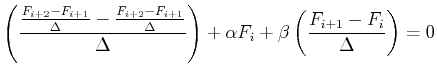
and then solve for the ``next increment'' $F_{i+2}$ if $F_{i+1}$ and $F_{i}$ are known.

Linear Differential Equations; Superposition in the Homogeneous Case

A linear differential equation is one for which the function and its derivatives are each linear--that is they appear in distinct terms and only to the first power. In the case of a homogeneous linear differential equation, the solutions are superposable. In other words, sums of solutions and their multiples are also solutions.

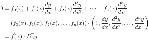
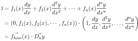
Therefore, a linear heterogeneous ordinary differential equation can be written as a product of general functions of the dependent variable and the derivatives for the $n$ -order linear case:

$$\begin{split}0 &= f_0(x) + f_1(x) \ensuremath{\frac{d{y}}{d{x... ...d{x}^{n}}}\right)\ &= \vec{f}(x) \cdot \vec{D_n y} \end{split}$$ (21-1)

The homogeneous $n^{th}$ -order linear ordinary differential equation is defined by $f_0(x)=0$ in Eq. 21-1:

$$\begin{split}0 &= f_1(x) \ensuremath{\frac{d{y}}{d{x}}} + f_2... ...n}}}\right)\ &= \vec{f_{hom}}(x) \cdot \vec{D_n y} \end{split}$$ (21-2)

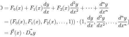
Equation 21-1 can always be multiplied by $1/f_n(x)$ to generate the general form:

$$\begin{split}0 &= F_0(x) + F_1(x) \ensuremath{\frac{d{y}}{d{x... ...}{y}}{d{x}^{n}}})\ &= \vec{F}(x) \cdot \vec{D_n y} \end{split}$$ (21-3)

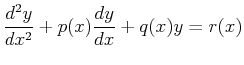
For the second-order linear ODE, the heterogeneous form can always be written as:

$$\ensuremath{\frac{d^2{y}}{d{x}^2}} + p(x) \ensuremath{\frac{d{y}}{d{x}}} + q(x) y = r(x)$$ (21-4)

and the homogeneous second-order linear ODE is:

$$\ensuremath{\frac{d^2{y}}{d{x}^2}} + p(x) \ensuremath{\frac{d{y}}{d{x}}} + q(x) y = 0$$ (21-5)

Basis Solutions for the homogeneous second-order linear ODE

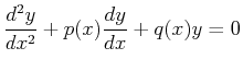
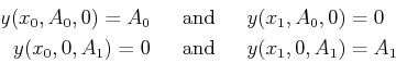
Because two values must be specified for each solution to a second order equation--the solution can be broken into two basic parts, each deriving from a different constant. These two independent solutions form a basis pair for any other solution to the homogeneous second-order linear ODE that derives from any other pair of specified values.

The idea is the following: suppose the solution to Eq. 21-5 is found the particular case of specified parameters $y(x=x_0) = A_0$ and $y(x=x_1) = A_1$ , the solution $y(x;A_0,A_1)$ can be written as the sum of solutions to two other problems.

$$y(x;A_0,A_1) = y(x,A_0,0) + y(x,0,A_1) = y_1(x) + y_2(x)$$ (21-6)

where

$$\begin{split}y(x_0,A_0,0) = A_0 & \text{\hspace{0.25in}and\hs... ...\hspace{0.25in}and\hspace{0.25in}} y(x_1,0,A_1)=A_1 \end{split}$$ (21-7)

from these two solutions, any others can be generated.

The two arbitrary integration constants can be included in the definition of the general solution:

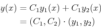$$\begin{split}y(x) &= C_1 y_1(x) + C_1 y_2(x)\ & = (C_1 , C_2) \cdot (y_1, y_2) \end{split}$$ (21-8)