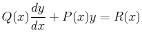
A linear differential equation is one that does not contain any powers (greater than one) of the function or its derivatives. The most general form is:
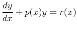
If ![]() , Eq. 20-15 is said to be a
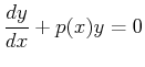
homogeneous linear first-order ODE; otherwise Eq. 20-15
is a heterogeneous linear first-order ODE.
, Eq. 20-15 is said to be a
homogeneous linear first-order ODE; otherwise Eq. 20-15
is a heterogeneous linear first-order ODE.
The reason that the homogeneous equation is linear is because solutions can
superimposed--that is, if ![]() and
and ![]() are solutions to
Eq. 20-15, then
are solutions to
Eq. 20-15, then
![]() is also a solution to
Eq. 20-15.
This is the case if the first derivative and the function are
themselves linear.
The heterogeneous equation is also called linear in this case,
but it is important to remember that sums and/or multiples of
heterogeneous solutions are also solutions to the heterogeneous equation.
is also a solution to
Eq. 20-15.
This is the case if the first derivative and the function are
themselves linear.
The heterogeneous equation is also called linear in this case,
but it is important to remember that sums and/or multiples of
heterogeneous solutions are also solutions to the heterogeneous equation.
The homogeneous equation has a solution of the form
| (20-16) |
|
MATHEMATICA |
| (notebook Lecture-20) |
| (html Lecture-20) |
| (xml+mathml Lecture-20) |
DSolve in Homogeneous and Heterogeneous ODEs
|
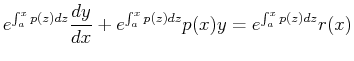
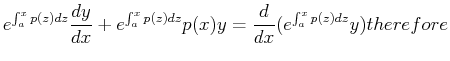
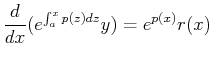
A trick (or, an integrating factor which amounts to the same thing)
can be employed to find the solution to the heterogeneous equation.
Multiply both sides of the heterogeneous
equation by
![]() :1
:1
 |
(20-17) |
 |
(20-18) |
 |
(20-19) |
![$\displaystyle y(x) = e^{-\int_a^x p(z) dz} \left[ \int_b^x r(z) \left( e^{\int_a^z p(\eta)d \eta}\right) dz \right]$](img67.png) |
(20-20) |