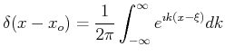
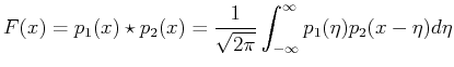
Because the inverse transform of a transform returns
the original function, this allows a definition of
an interesting function called the Dirac delta function
![]() .
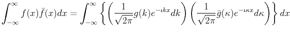
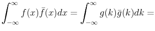
Combining the two equations in Eq. 18-5 into
a single equation, and then interchanging the order of integration:
.
Combining the two equations in Eq. 18-5 into
a single equation, and then interchanging the order of integration:
 |
(18-8) |
 |
(18-9) |
 |
(18-10) |
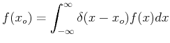
The delta function can be used to derive an important conservation theorem.
If ![]() represents the density of some function (i.e., a
wave-function like
represents the density of some function (i.e., a
wave-function like ![]() ), the square-magnitude of
), the square-magnitude of ![]() integrated
over all of space should be the total amount of material in
space.
integrated
over all of space should be the total amount of material in
space.
 |
(18-11) |
 |
(18-12) |
 |
(18-13) |
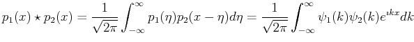
The proof is straightforward that the convolution of
two functions, ![]() and
and ![]() , is a Fourier integral over the product
of their Fourier transforms,
, is a Fourier integral over the product
of their Fourier transforms, ![]() and
and ![]() :
:
 |
(18-14) |
Another way to think of this is that ``the net effect on the spatial function due two interfering waves is contained by product the fourier transforms.'' Practically, if the effect of an aperture (i.e., a sample of only a finite part of real space) on a wave-function is desired, then it can be obtained by multiplying the Fourier transform of the aperture and the Fourier transform of the entire wave-function.
|
MATHEMATICA |
| (notebook Lecture-18) |
| (html Lecture-18) |
| (xml+mathml Lecture-18) |
|
Creating Lattices for Subsequent Fourier Transform
A diffraction pattern from a group of scattering centers such atoms is related to the Fourier transform of the ``atom'' positions:
|
|
MATHEMATICA |
| (notebook Lecture-18.nb) |
| (html Lecture-18.nb) |
| (xml+mathml Lecture-18.nb) |
| Discrete Fourier Transforms
A Fourier transform is over an infinite domain. Numerical data is seldom infinite, therefore a strategy must be applied to get a Fourier transform of data. Discrete Fourier transforms (DFT) operate by creating a lattice of copies of the original data and then returning the Fourier transform of the result. Symmetry elements within the data appear in the Discrete Fourier transform and are superimposed with the Transform of the symmetry operations due to the virtual infinite lattice of data patterns.
Because there are a finite number of pixels in the
data, there are also the same finite number of sub-periodic
wave-numbers that can be determined.
In other words, the Discrete Fourier Transform of
a
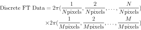
representing the amplitudes of the indicated periodicities.
|
|
MATHEMATICA |
| (notebook Lecture-18.nb) |
| (html Lecture-18.nb) |
| (xml+mathml Lecture-18.nb) |
| Fourier Transforms on Lattices with Thermal Noise
Lattices in real systems not only contain defects, but also some uncertainty in the positions of the atoms because of thermal effects such as phonons.
|
|
MATHEMATICA |
| (notebook Lecture-18.nb) |
| (html Lecture-18.nb) |
| (xml+mathml Lecture-18.nb) |
| Imaging from Selected Regions of Reciprocal Space
To select and interpret different regions of Fourier space, a function will be produced that selects a particular region of the Fourier Space (i.e., as selected set of possible periodicities) and then visualize the Back-Transform of only that region.
|
|
MATHEMATICA |
| (notebook Lecture-18.nb) |
| (html Lecture-18.nb) |
| (xml+mathml Lecture-18.nb) |
| Taking Discrete Fourier Transforms of Images
A image in graphics format, such as a .gif, contains
intensity as a function of position.
If the function is gray-scale data, then each pixel typically
takes on
|