Expansion of a function in terms of Fourier Series proved to
be an effective way to represent functions that were periodic
in an interval
![]() .
Useful insights into ``what makes up a function'' are obtained
by considering the amplitudes of the harmonics (i.e., each of
the sub-periodic trigonometric or complex oscillatory functions)
that compose the Fourier series.
That is, the component harmonics can be quantified
by inspecting their amplitudes.
For instance, one could quantitatively compare the same note generated from
a Stradivarius to an ordinary violin by comparing the amplitudes
of the Fourier components of the notes component frequencies.
.
Useful insights into ``what makes up a function'' are obtained
by considering the amplitudes of the harmonics (i.e., each of
the sub-periodic trigonometric or complex oscillatory functions)
that compose the Fourier series.
That is, the component harmonics can be quantified
by inspecting their amplitudes.
For instance, one could quantitatively compare the same note generated from
a Stradivarius to an ordinary violin by comparing the amplitudes
of the Fourier components of the notes component frequencies.
However there are many physical examples of phenomena that involve nearly, but not completely, periodic phenomena--and of course, quantum mechanics provides many examples of isolated events that are composed of wave-like functions.
It proves to be very useful to extend the Fourier analysis to functions that are not periodic. Not only are the same interpretations of contributions of the elementary functions that compose a more complicated object available, but there are many others to be obtained.
To extend Fourier series to non-periodic functions, the domain
of periodicity will extended to infinity, that is the limit
of
![]() will be considered.
This extension will be worked out in a heuristic manner in this
lecture--the formulas will be correct, but the rigorous details
are left for the math textbooks.
will be considered.
This extension will be worked out in a heuristic manner in this
lecture--the formulas will be correct, but the rigorous details
are left for the math textbooks.
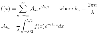
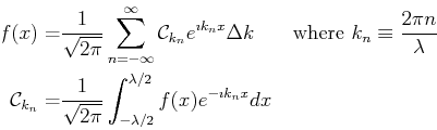
Recall that the complex form of the Fourier series was written as:
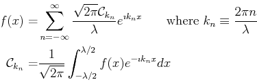
This can be written in a more symmetric form by scaling the amplitudes
with ![]() --let
--let
![]() , then
, then
 |
(18-2) |
 |
(18-3) |
 |
(18-4) |
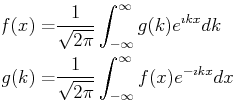
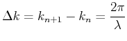
Now, the limit
![]() can be obtained an the
summation becomes an integral over a continuous spectrum of wave-numbers;
the amplitudes become a continuous function of wave-numbers,
can be obtained an the
summation becomes an integral over a continuous spectrum of wave-numbers;
the amplitudes become a continuous function of wave-numbers,
![]() :
:
The Fourier transform that integrates
![]() over
all
over
all ![]() can
be extended straightforwardly to a two dimensional integral
of a function
can
be extended straightforwardly to a two dimensional integral
of a function
![]() by
by
![]() over all
over all ![]() and
and ![]() --or to a three-dimensional
integral of
--or to a three-dimensional
integral of
![]() over an infinite three-dimensional
volume.
over an infinite three-dimensional
volume.
A wavenumber appears for each new spatial
direction and they represent the periodicities in the
![]() -,
-, ![]() -, and
-, and ![]() -directions.
It is natural to turn the wave-numbers into a wave-vector
-directions.
It is natural to turn the wave-numbers into a wave-vector
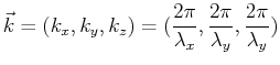 |
(18-6) |
The three dimensional Fourier transform pair takes the form:
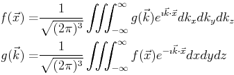 |
(18-7) |