Next: Stokes' Theorem
Up: Lecture_16_web
Previous: Higher-dimensional Integrals
Next: Stokes' Theorem
Up: Lecture_16_web
Previous: Higher-dimensional Integrals
Suppose there is ``stuff'' flowing from place to place in three
dimensions.
Figure:
Illustration of a vector ``flow field''  near
a point in three dimensional space.
If each vector represents the rate of ``stuff'' flowing per unit area
of a plane that is normal to the direction of flow, then the
dot product of the flow field integrated over a planar oriented area
near
a point in three dimensional space.
If each vector represents the rate of ``stuff'' flowing per unit area
of a plane that is normal to the direction of flow, then the
dot product of the flow field integrated over a planar oriented area  is the rate of ``stuff'' flowing through that plane.
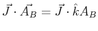
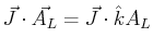
For example, consider the two areas indicated with purple (or dashed) lines.
The rate of ``stuff'' flowing through those regions is
is the rate of ``stuff'' flowing through that plane.
For example, consider the two areas indicated with purple (or dashed) lines.
The rate of ``stuff'' flowing through those regions is
 and
and
 .
.

|
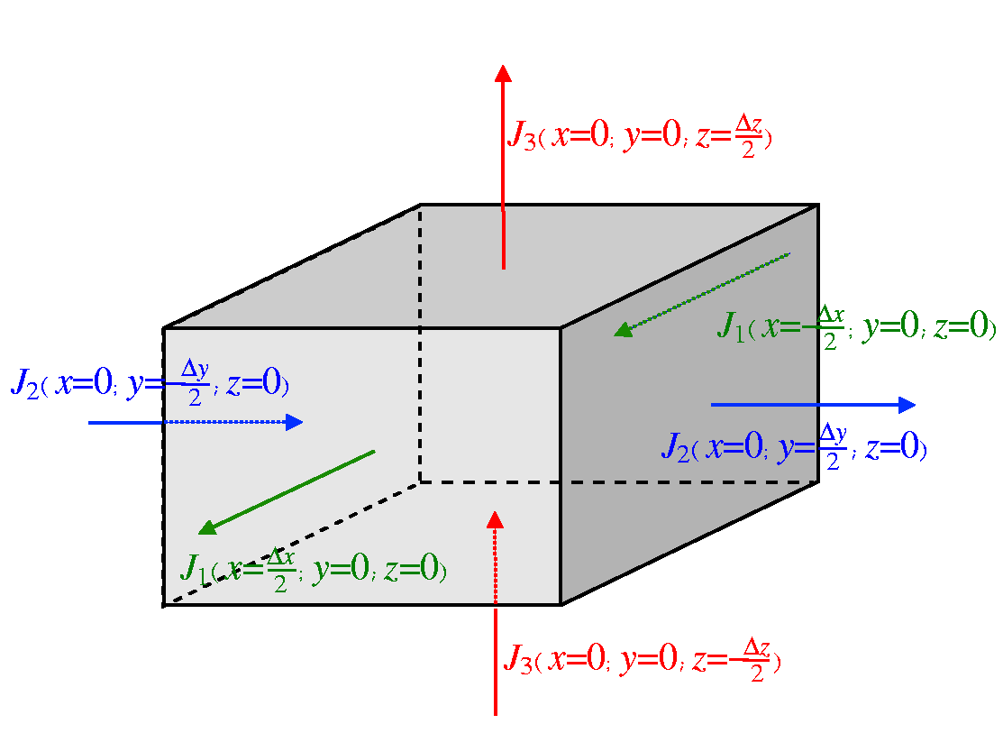
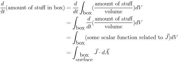
If there are no sources or sinks that create or destroy stuff
inside a small box surrounding a point, then the change in the
amount of stuff in the
volume of the box must be related to some integral over the box's surface:
 |
(16-1) |
Figure 16-4:
Integration of a vector function near
a point and its relation to the change in that vector function.
The rate of change of stuff is the integral of flux over the
outside--and
in the limit as the box size goes to zero, the rate of change of
the amount of stuff is related to the sum of derivatives of the
flux components at that point.
|
|
To relate the rate at which ``stuff  '' is flowing into a small
box of volume
'' is flowing into a small
box of volume
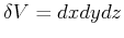 located at
  due to
a flux
,
note that the amount that
changes in a time
due to
a flux
,
note that the amount that
changes in a time  is:
is:
 |
(16-2) |
If
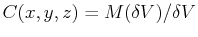 is the concentration (i.e., stuff per volume) at
, then
in the limit of small volumes and short times:
is the concentration (i.e., stuff per volume) at
, then
in the limit of small volumes and short times:
 div div |
(16-3) |
For an arbitrary closed volume  bounded by an oriented surface
 :
:
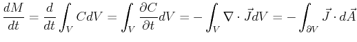 |
(16-4) |
The last equality
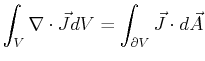 |
(16-5) |
is called the Gauss or the divergence theorem.
© W. Craig Carter 2003-, Massachusetts Institute of Technology