Link to Current (updated) notes

next previous Next: Integration over Surfaces Up: Lecture_15_web Previous: Green's Theorem for Area in Plane Relating to

Representations of Surfaces

Integration over the plane $ z=0$ in the form of $ \int f(x,y) dx dy$ introduces surface integration--over a planar surface--as a straightforward extension to integration along a line. Just as integration over a line was generalized to integration over a curve by introducing two or three variables that depend on a single variable (e.g., $ (x(t),y(t),z(t))$ ), a surface integral can be conceived as introducing three (or more) variables that depend on two parameters (i.e., $ (x(u,v), y(u,v), z(u,v))$ ).

However, there are different ways to formulate representations of surfaces:

MATHEMATICA$ ^{\text{\scriptsize {\textregistered }}}$ Example
(notebook Lecture-15)
(html Lecture-15)
(xml+mathml Lecture-15)
Representations of Surfaces

Surfaces and interfaces play fundamental roles in materials science and engineering. Unfortunately, the mathematics of surfaces and interfaces frequently presents a hurdle to materials scientists and engineering. The concepts in surface analysis can be mastered with a little effort, but there is no escaping the fact that the algebra is tedious and the resulting equations are onerous. Symbolic algebra and numerical analysis of surface alleviates much of the burden.

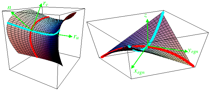
Most of the practical concepts derive from a second-order Taylor expansion of a surface near a point. The first-order terms define a tangent plane; the tangent plane determines the surface normal. The second-order terms in the Taylor expansion form a matrix and a quadratic form that can be used to formulate an expression for curvature. The eigenvalues of the second-order matrix are of fundamental importance.

The Taylor expansion about a particular point on the surface takes a particularly simple form if the origin of the coordinate system is located at the point and the $ z$ -axis is taken along the surface normal as illustrated in the following figure.

surfaces.png
Figure: Parabolic approximation to a surface and local eigenframe. The surface on the left is a second-order approximation of a surface at the point where the coordinate axes are drawn. The surface has a local normal at that point which is related to the cross product of the two tangents of the coordinate curves that cross at the that point. The three directions define a coordinate system. The coordinate system can be translated so that the origin lies at the point where the surface is expanded and rotated so that the normal $ \hat{n}$ coincides with the $ z$ -axis as in the right hand curve.
\resizebox{6in}{!}
{\includegraphics{figures/newbar.eps}}

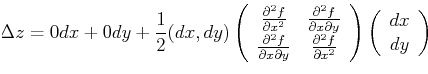
In this coordinate system, the Taylor expansion of $ z= f(x,y)$ must be of the form

\begin{displaymath}
\Delta z = 0 dx + 0 dy + \frac{1}{2}(dx,dy)
\left(
\begin{ar...
...ay}\right)
\left(
\begin{array}{c}
dx\\
dy
\end{array}\right)
\end{displaymath}

If this coordinate system is rotated about the $ z$ -axis into its eigenframe where the off-diagonal components vanish, then the two eigenvalues represent the maximum and minimum curvatures. The sum of the eigenvalues is invariant to transformations and the sum is known as the mean curvature of the surface. The product of the eigenvalues is also invariant--this quantity is known as the Gaussian curvature.

The method in the figure suggests a method to calculate the normals and curvatures for a surface. Those results are tabulated below.

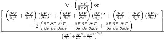
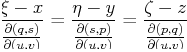
Level Set Surfaces: Tangent Plane, Surface Normal, and Curvature
\begin{center}\vbox{\input{LectureTopics/level-set-surface.tex}
}\end{center}
Tangent Plane ( $ \vec{x} = (x,y,z)$ , $ \vec{\xi} =(\xi , \eta, \zeta)$ )
\begin{center}\vbox{\input{LectureTopics/level-set-tangent.tex}
}\end{center}
Normal
\begin{center}\vbox{\input{LectureTopics/level-set-normal.tex}
}\end{center}
Mean Curvature
\begin{center}\vbox{\input{LectureTopics/level-set-curvature.tex}
}\end{center}

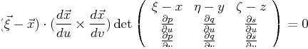
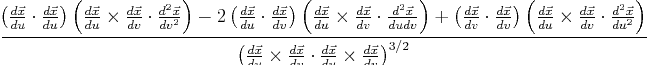
Parametric Surfaces: Tangent Plane, Surface Normal, and Curvature
\begin{center}\vbox{\input{LectureTopics/parametric-surface.tex}
}\end{center}
Tangent Plane ( $ \vec{x} = (x,y,z)$ , $ \vec{\xi} =(\xi , \eta, \zeta)$ )
\begin{center}\vbox{\input{LectureTopics/parametric-tangent.tex}
}\end{center}
Normal
\begin{center}\vbox{\input{LectureTopics/parametric-normal.tex}
}\end{center}
Mean Curvature
\begin{center}\vbox{\input{LectureTopics/parametric-curvature.tex}
}\end{center}

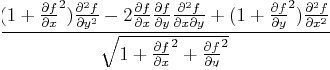
Graph Surfaces: Tangent Plane, Surface Normal, and Curvature
\begin{center}\vbox{\input{LectureTopics/graph-surface.tex}
}\end{center}
Tangent Plane ( $ \vec{x} = (x,y,z)$ , $ \vec{\xi} =(\xi , \eta, \zeta)$ )
\begin{center}\vbox{\input{LectureTopics/graph-tangent.tex}
}\end{center}
Normal
\begin{center}\vbox{\input{LectureTopics/graph-normal.tex}
}\end{center}
Mean Curvature
\begin{center}\vbox{\input{LectureTopics/graph-curvature.tex}
}\end{center}


© W. Craig Carter 2003-, Massachusetts Institute of Technology