Link to Current (updated) notes

Green's Theorem for Area in Plane Relating to its Bounding Curve

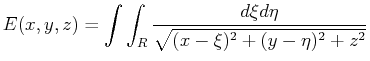
Reappraise the simplest integration operation, $g(x) = \int f(x) dx$ . Temporarily ignore all the tedious mechanical rules of finding and integral and concentrate on what integration does.

Integration replaces a fairly complex process--adding up all the contributions of a function $f(x)$ --with a clever new function $g(x)$ that only needs end-points to return the result of a complicated summation.

It is perhaps initially astonishing that this complex operation on the interior of the integration domain can be incorporated merely by the domain's endpoints. However, careful reflection provides a counterpoint to this marvel. How could it be otherwise? The function $f(x)$ is specified and there are no surprises lurking along the $x$ -axis that will trip up $dx$ as it marches merrily along between the endpoints. All the facts are laid out and they willingly submit to the process their preordination by $g(x)$ by virtue of the endpoints.¹

The idea naturally translates to higher dimensional integrals and these are the basis for Green's theorem in the plane, Stoke's theorem, and Gauss (divergence) theorem. Here is the idea:

Figure 15-1: An irregular region on a plane surrounded by a closed curve. Once the closed curve (the edge of region) is specified, the area inside it is already determined. This is the simplest case as the area is the integral of the function $f=1$ over $dx dy$ . If some other function, $f(x,y)$ , were specified on the plane, then its integral is also determined by summing the contributions along the boundary. This is a generalization $g(x) = \int f(x) dx$ and the basis behind Green's theorem in the plane.

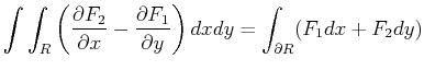
The analog of the ``Fundamental Theorem of Differential and Integral Calculus''² for a region $\mathcal{R}$ bounded in a plane with normal $\hat{k}$ that is bounded by a curve $\partial \mathcal{R}$ is:

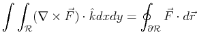$$\int \int_{\mathcal{R}} (\nabla \times \vec{F}) \cdot \hat{k} dx dy = \oint_{\partial \mathcal{R}} \vec{F} \cdot d \vec{r}$$ (15-1)

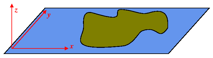
The following figure motivates Green's theorem in the plane:

Figure 15-2: Illustration of how a vector valued function in a planar domain "spills out" of domain by evaluating the curl everywhere in the domain. Within the domain, the rotational flow ( $\ensuremath{\nabla}\times F$ ) from one cell moves into its neighbors; however, at the edges the local rotation is a net loss or gain. The local net loss or gain is $\vec{F} \cdot (dx,dy)$ .

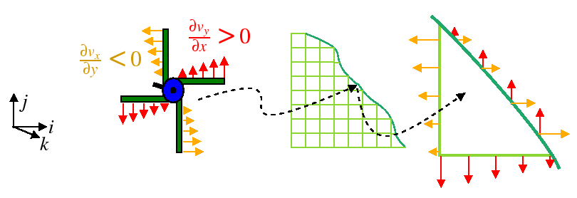
The generalization of this idea to a surface $\partial \mathcal{B}$ bounding a domain $\mathcal{B}$ results in Stokes' theorem, which will be discussed later.

MATHEMATICA$^{\text{\scriptsize {\textregistered }}}$ Example

(notebook Lecture-15)

(html Lecture-15)

(xml+mathml Lecture-15)

Turing an integral over a domain into an integral over its boundary Using Green's theorem in the plane to simplify the integration to find the potential above a triangular path that was evaluated in the last lecture.

Here we turn the two dimensional numerical integration which requires $\mathcal{O}(N^2)$ calculations into an integration around the boundary which requires $\mathcal{O}(N)$ evaluations for the same accuracy.

1. The integral in question is:
   $$E(x,y,z) = \int \int_{R} \frac{d \xi d \eta} {\sqrt{(x-\xi)^2 + (y-\eta)^2 + z^2}}$$

2. Green's theorem in the plane is:
   $$\int \int_{R} \left( \ensuremath{\frac{\partial{F_2}}{\partial{x}... ...artial{F_1}}{\partial{y}}} \right) dxdy = \int_{\partial R} ( F_1 dx + F_2 dy)$$

3. Find a function $\vec{F} = (F_1 , F_2)$ which matches the integral in questions. This can be done by simply setting $F_2 = 0$ and integrating to find $F_1$
   $$F_1 = \int \frac{d \eta} {\sqrt{(x-\xi)^2 + (y-\eta)^2 + z^2}}$$
   which not very difficult.
4. It remains to parameterize the three legs of the triangle as paths to integrate over (i.e., use $(x(t), y(t))$ from the three line segments and integrate over $(dx,dy) = (x'dt, y'dt)$ .
5. The integral is still to complicated, however the numerical evaluation of this boundary integral is much more efficient.