Link to Current (updated) notes

Quadratic Forms

The example above, where a matrix (rank-2 tensor) represents a material property, can be understood with a useful geometrical interpretation.

For the case of the conductivity tensor $\mat {\sigma}$ , the dot product $\vec{E} \cdot \vec{j}$ is a scalar related to the local energy dissipation:

$$e = \vec{E}^T \mat {\sigma} \vec{E}$$ (10-21)

The term on the right-hand-side is called a quadratic form, as it can be written as:

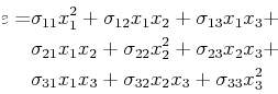$$\begin{split}e = & \sigma_{11} x_1^2 + \sigma_{12} x_1 x_2 + ... ...} x_1 x_3 + \sigma_{32} x_2 x_3 + \sigma_{33} x_3^2 \end{split}$$ (10-22)

or, because $\mat {\sigma}$ is symmetric:

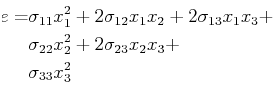$$\begin{split}e = & \sigma_{11} x_1^2 + 2\sigma_{12} x_1 x_2 +... ..._2^2 + 2 \sigma_{23} x_2 x_3 +\ &\sigma_{33} x_3^2 \end{split}$$ (10-23)

It is not unusual for such quadratic forms to represent energy quantities. For the case of paramagnetic and diamagnetic materials with magnetic permeability tensor $\mat {\mu}$ , the energy per unit volume due to an applied magnetic field $\vec{H}$ is:

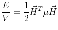$$\frac{E}{V} = \frac{1}{2} \vec{H}^T \mat {\mu} \vec{H}$$ (10-24)

for a dielectric (i.e., polarizable) material with electric electric permittivity tensor $\mat {\kappa}$ with an applied electric field $\vec{E}$ :

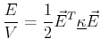$$\frac{E}{V} = \frac{1}{2} \vec{E}^T \mat {\kappa} \vec{E}$$ (10-25)

The geometric interpretation of the quadratic forms is obtained by turning the above equations around and asking--what are the general vectors $\vec{x}$ for which the quadratic form (usually an energy or power density) has a particular value? Picking that particular value as unity, the question becomes what are the directions and magnitudes of $\vec{x}$ for which

$$1 = \vec{x}^T \mat {A} \vec{x}$$ (10-26)

This equation expresses a quadratic relationship between one component of $\vec{x}$ and the others. This is a surface--known as the quadric surface or representation quadric--which is an ellipsoid or hyperboloid sheet on which the quadratic form takes on the particular value 1.

In the principal axes (or, equivalently, the eigenbasis) the quadratic form takes the quadratic form takes the simple form:

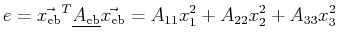$$e = \vec{x_{\text{eb}}}^T \mat {A_{\text{eb}}} \vec{x_{\text{eb}}} = A_{11} x_1^2 + A_{22} x_2^2 + A_{33} x_3^2$$ (10-27)

and the representation quadric

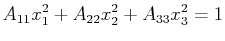$$A_{11} x_1^2 + A_{22} x_2^2 + A_{33} x_3^2 = 1$$ (10-28)

which is easily characterized by the signs of the coefficients.

In other words, in the principal axis system (or the eigenbasis) the quadratic form has a particularly simple, in fact the most simple, form.