In many applications, the coordinate system (or laboratory) frame of the vector that gets operated on is the same as the vector gets returned. This is the case for almost all physical properties. For example:
| (10-1) |
| (10-2) |
| (10-3) |
| (10-4) |
When ![]() and
and ![]() are vectors representing a
physical quantity in Cartesian space (such as force
are vectors representing a
physical quantity in Cartesian space (such as force
![]() , electric field
, electric field ![]() , orientation of
a plane
, orientation of
a plane ![]() , current
, current ![]() , etc.) they represent
something physical.
They don't change if we decide to use a different space in which
to represent them (such as, exchanging
, etc.) they represent
something physical.
They don't change if we decide to use a different space in which
to represent them (such as, exchanging ![]() for
for ![]() ,
, ![]() for
for ![]() ,
, ![]() for
for ![]() ;
or, if we decide to represent length in nanometers instead of inches, or
if we simply decide to rotate the system that describes the vectors.
The representation of the vectors themselves may change, but they
stand for the same thing.
;
or, if we decide to represent length in nanometers instead of inches, or
if we simply decide to rotate the system that describes the vectors.
The representation of the vectors themselves may change, but they
stand for the same thing.
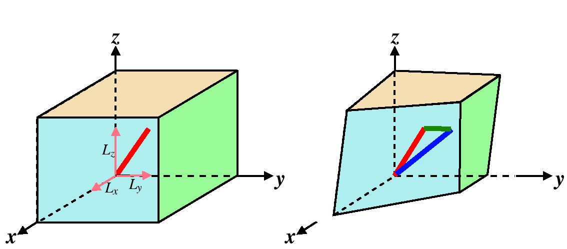
One interpretation of the operation
![]() has been described as geometric transformation on the vector
has been described as geometric transformation on the vector ![]() .
For the case of orthogonal matrices
.
For the case of orthogonal matrices
![]() , geometrical
transformations take the forms of rotation, reflection, and/or inversion.
, geometrical
transformations take the forms of rotation, reflection, and/or inversion.
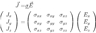
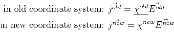
Suppose we have some physical relation between two physical vectors in some coordinate system, for instance, the general form of Ohm's law is:
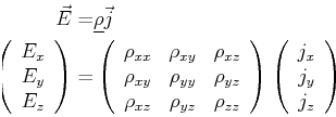
The physical law in Eq. 10-5 can be expressed as an inverse relationship:
What happens if we decide to use a new coordinate system (i.e., one that is rotated, reflected, or inverted) to describe the relationship expressed by Ohm's law?
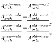
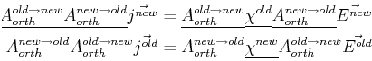
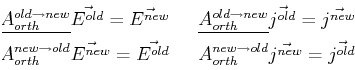
The two vectors must transform from the ``old'' to the ``new'' coordinates by:
 |
(10-8) |
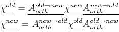
How does the physical law expressed by Eq. 10-5 change in a new coordinate system?
| (10-10) |
| (10-11) |
 |
(10-12) |
The
![]() is said to be similar to
is said to be similar to
![]() and the double
multiplication operation in Eq. 10-13 is called a similarity transformation.
and the double
multiplication operation in Eq. 10-13 is called a similarity transformation.
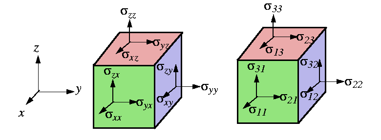
Stresses and strains are rank-2 tensors that characterize the mechanical state of a material.
A spring is an example of a one-dimensional material--it resists or exerts force in one direction only. A volume of material can exert forces in all three directions simultaneously--and the forces need not be the same in all directions. A volume of material can also be ``squeezed'' in many different ways: it can be squeezed along any one of the axis or it can be subjected to squeezing (or smeared) around any of the axes1
All the ways that a force can be applied to small element of material are now described. A force divided by an area is a stress--think of it the areal density of force.
There is one special and very simple case of elastic stress, and that is
called the hydrostatic stress.
It is the case of pure pressure and there are no shear (off-diagonal) stresses
(i.e., all
![]() for
for ![]() , and
, and
![]() ).
An equilibrium system composed of a body in a fluid environment is always in hydrostatic stress:
).
An equilibrium system composed of a body in a fluid environment is always in hydrostatic stress:
Strain is also a rank-2 tensor and it is a physical measure of a how much a material changes its shape.2
Why should strain be a rank-2 tensor?
|
|
Or, using the same idea as that for stress:
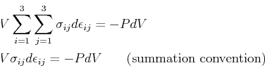
If a body that is being stressed hydro-statically is isotropic, then its response is pure dilation (in other words, it expands or shrinks uniformly and without shear):
So, for the case of hydrostatic stress, the work term has a particularly simple form:
This expression is the same as the rate of work performed on a compressible fluid, such as an ideal gas.
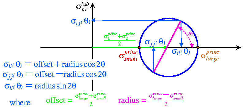
For any stress matrix, there is a choice of an coordinate system where all shear stresses (the off-diagonal terms) vanish and the matrix is diagonal.
These coordinate systems define the eigenstrain and eigenstress. The matrix transformation that takes a coordinate system into its eigenstate is of great interest because it simplifies the mathematical representation of the physical system.
|
MATHEMATICA |
| (notebook Lecture-10) |
| (html Lecture-10) |
| (xml+mathml Lecture-10) |
| Principal Axes
|
|
|
 (i.e.,
 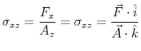 )
)![$\displaystyle \sigma_{ij} = \left[ \begin{array}{ccc} \sigma_{xx} & \sigma_{xy}...
...y} & \sigma_{yz} \ \sigma_{zx} & \sigma_{zy} & \sigma_{zz} \end{array} \right]$](img41.png)
![$\displaystyle \sigma_{ij} = \left[ \begin{array}{ccc} -P & 0 & 0 \ 0 & -P & 0 \ 0 & 0 & -P \end{array} \right]$](img45.png)
 (i.e.,
  )
)![$\displaystyle \epsilon_{ij} = \left[ \begin{array}{ccc} \Delta/3 & 0 & 0 \ 0 & \Delta/3 & 0 \ 0 & 0 & \Delta/3 \end{array} \right]$](img49.png)