Last time we introduced two different kinds of thermodynamic variables: Extensive and Intensive
Intensive variables can be specified point by point; i.e.
They do not depend on the size of the body.
Extensive variables depend on the size of the system in question. They are additive.
 |
(04-4) |
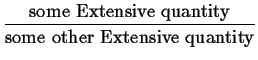
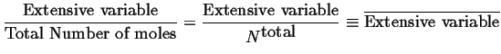
We can define ``derived quantities'' (or densities) by scaling:1
 |
(04-5) |
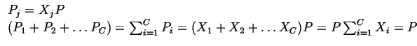
However, the derived intensive quantities still `act' like extensive quantities regarding where they appear in `work' terms:
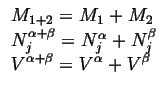
Extensive variables can be distinguished from intensive variables by the way
they add when you add two systems at equilibrium (See Eq. ![[*]](crossref.gif) ).
Derived quantities don't sum like extensive or intensive quantities, but one
can derive a rule for their addition.
The trick in involves realizing that the derived quantities are ``extensive variables
in hiding.''
One can turn them into extensive variables and then use the appropriate rule to add,
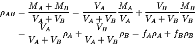
for instance, consider the combined density,
).
Derived quantities don't sum like extensive or intensive quantities, but one
can derive a rule for their addition.
The trick in involves realizing that the derived quantities are ``extensive variables
in hiding.''
One can turn them into extensive variables and then use the appropriate rule to add,
for instance, consider the combined density,
![]() of two bodies with volumes
of two bodies with volumes
![]() ,
,
![]() , and masses
, and masses
![]() ,
,
![]() :
:
 |
(04-6) |
Examples of derived intensive quantities are:
 |
(04-7) |
 |
(04-8) |
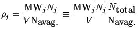
This last equation introduces another derived intensive quantity called a molar quantity:
 |
(04-9) |
For example, molar species number
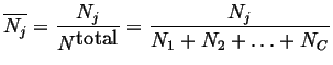 |
(04-10) |
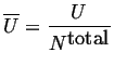 |
(04-11) |
![]()
Partial Quantities
For intensive quantities, it is sometimes useful to associate the contributions of each type of existing chemical species to the value of the intensive quantities. Each separate contribution is called a partial quantity, for example for pressure,
 |
(04-12) |
![]() is defined as the partial pressure of species
is defined as the partial pressure of species
![]()
Question: Does the product of two extensive variables produce a similar extensive variable?
Question: Does the product of two intensive variables produce an intensive variable?
Question: Under what conditions does the product of an intensive variable and an extensive variable produce an extensive variable?