The code for this particular application (which can be found in 8 ) was written in less than one hour; a fairly accurate solution is obtained in about 30 seconds on a medium speed workstation.
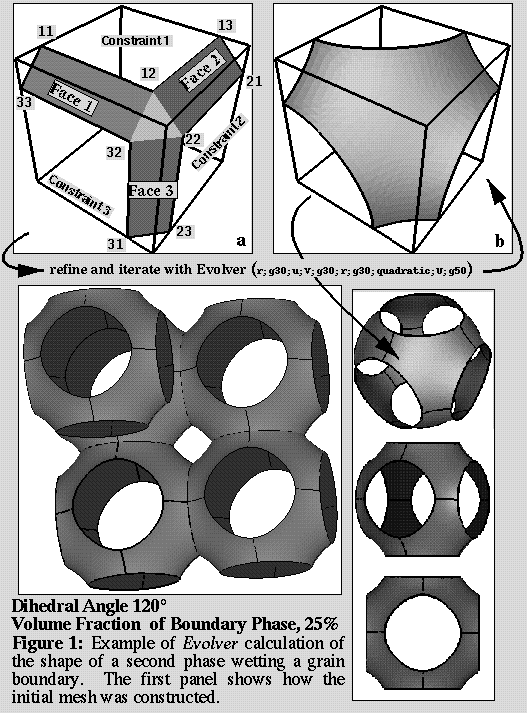
The object is to calculate the shape of a fixed volume second phase which lies along the triple junctions of grains composed of a primary phase. The second phase forms a dihedral angle at the grain boundaries. If the second phase is gas phase (say, a vapor in equilibrium with the primary phase), this would be a good geometric model of a sintering body.
However, the arrangement of grains is somewhat unrealistic. The unit cell (primary phase in center plus grain boundary phase along the edges) for each grain was chosen as a rectangular prism to simplify the Evolver code. It is reasonably straightforward to set up the case where the grains are tetrakaidecahedra.
The method by which the code in 8 was developed can be briefly summarized. The model variables were determined. Account was made of various surfaces which were known to be important; in this case, the grain boundary and primary-secondary interface. Symmetries which were available were used to simplify the coding. Some vector potentials (described below in detail) were determined by ``intelligent guessing'' them and verifying the result. For the initial mesh, a picture was sketched by hand and the vertices, edges and facets where assigned. Several Evolver runs are made and adjustments are made to the surface mesh by visual inspection.
Please refer to Figure 1 for a graphic description of the code in 8.
Note that Evolver comments have the C++ syntax (e.g, they are preceded by
![]() or begin with
or begin with ![]() and end with
and end with ![]()
The Evolver code initializes parameters which may considered to make up a three-parameter family of interesting boundary phase shapes: the volume fraction of the primary phase, the dihedral angle, and the cell height. All these parameters can be changed any time during an Evolver session.
Next, various functions or useful quantities are defined. The functions can depend on the parameters; adjusting a parameter changes the value of a function during an Evolver session. The width and depth of the cell are defined so that total cell volume is unity; this could be easily generalized by defining more parameters. The effective tension is the difference in energy per unit area created by uncovering area on the constraint. The surface tension of the primary/secondary interface is unity. The offset is a parameter which is useful in setting up the intial mesh, described below.
The symmetry of the rectangular prism unit cell is used to advantage.
![]() Only the upper octant is modeled.
Generators of the symmetry group are introduced only to view the
entire cell graphically.
Only the upper octant is modeled.
Generators of the symmetry group are introduced only to view the
entire cell graphically.
Six constraints are specified in this Evolver code: three cell walls, where the grain boundaries are located, and three mirror planes.
Consider constraint 1 (Figure 1). The constraint is given as the formula, z = height. Since the grain boundary is flat and since we would like to avoid putting facets on the grain boundary (see reasons given above), a method for accounting for the energy is required. the following stratagem is used (this trick is ubiquitous in Evolver ): The energy of the grain boundary on constraint 1 is given by:
![]()
where ![]() is the unit vector parallel to the z direction
and
is the unit vector parallel to the z direction
and ![]() is an element of area on the constraint.
is an element of area on the constraint.
If the closed curve which surrounds ![]() (call it
(call it ![]() , the
boundary curve) is known, then it follows that
, the
boundary curve) is known, then it follows that ![]() should be determined
from that curve.
This is just a statement of a fundamental theorem from vector calculus:
should be determined
from that curve.
This is just a statement of a fundamental theorem from vector calculus:
where ![]() is a directed line element on the boundary curve
is a directed line element on the boundary curve ![]() .
.
The task at hand is to find any ![]() such
that
such
that ![]() .
For planar problems like this, one choice is
.
For planar problems like this, one choice is
![]() .
That vector potential becomes input for the energy: definition
of that constraint and we leave it up to Evolver to use those edges
on constraint 1 as the
.
That vector potential becomes input for the energy: definition
of that constraint and we leave it up to Evolver to use those edges
on constraint 1 as the ![]() parts of a discrete approximation
to an integral of
parts of a discrete approximation
to an integral of ![]() over all the
edges on the constraint.
over all the
edges on the constraint.
There is also volume content associated with constraint 1. One way that Evolver calculates can calculate volume is simply account for the volume between a facet and its projection on the z=0 plane. However there are no facets on constraint 1, so we must account for the volume by using the edges lying on the constraint.
The same trick is applied yet again to find the volume under the grain boundary:
where the vector field ![]() is chosen so
that
is chosen so
that ![]() .
There are many such choices for
.
There are many such choices for ![]() , a simple choice is:
, a simple choice is:
![]() , in fact this is the one that Evolver
uses as the default for the volume below a facet.
, in fact this is the one that Evolver
uses as the default for the volume below a facet.
![]() The last integral of Equation 3 looks like the first integral of
Equation 2, so we should try to find vector field
The last integral of Equation 3 looks like the first integral of
Equation 2, so we should try to find vector field ![]() such that
such that ![]() .
However, it is not so straightforward since for any vector field
.
However, it is not so straightforward since for any vector field ![]()
![]() , and we have specifically
picked
, and we have specifically
picked ![]() so that
so that ![]() !
The trick is to convert
!
The trick is to convert ![]() into an equivalent
divergenceless form on the constraint:
into an equivalent
divergenceless form on the constraint:
![]() .
Therefore, an
.
Therefore, an ![]() can be found,
can be found, ![]() and that is what is written into the Evolver file as
and that is what is written into the Evolver file as ![]() .
.
The other grain boundaries, constraint 2 and constraint 3, have
similar terms for the energy vector integrand, but do not contribute any
extra volume content since each one has a normal which is perpendicular
to ![]() .
.
The other mirror planes contribute neither energy nor content.
Note that contributing no energy is equivalent to setting the dihedral angle
to ![]() : where it intersects, the surface is perpendicular to the mirror plane.
: where it intersects, the surface is perpendicular to the mirror plane.
Next, the geometry and connectivity of an initial surface is delineated. Referring to Figure 1, the vertices are "named" with a integer index. The index can be any positive integer (but smaller that the largest integer that your computer will read, of course) and it is useful to give elements indices that helps the user associate them. The coordinates of the vertices are given and the constraints on which they lie.
The edges are also given by an index and the vertices that define their beginning and end. The constraints not only specify a surface that the edge will lie upon (as well as any new edges which inherit that constraint as the edge is subdivided) but also specify that vector integrands be performed as required by the constraint. Here the edge indices are chosen here in an obvious manner which is not only useful, but aid in debugging their ordering on the face list.
Faces are given by an index plus an ordered list of oriented edges. It is useful to color the faces so that they can be graphically distinguished. Faces that have more than three edges are automatically subdivided by Evolver .
The bodies are given by an index plus a list of all of its faces and a volume may also be specified. The additional surfaces which bound the body are implied by the edges which lie on the constraint which are also members of faces in the face list.
Finally the program can be run. If the Evolver code given above is in a file called boundary_phase.fe it is typically executed by typing evolver boundary_phase.fe at a computer prompt. It is essential to use graphics of some sort. Refer to the manual that comes with the Evolver source for details for particular computer systems.
To produce the result given in Figure 1, the following Evolver commands were given r; g30 ; u ; V ; g30 ; r ; g30 ; quadratic ; U ; g50; which means: 1) r refine the surface mesh by subdividing the edges, 2) g30 go 30 iterations by moving each vertex in a direction parallel to its local gradient, 3) u adjust the mesh by making edge switches to make facets more equilateral, 4) V adjust the mesh by vertex averaging, this tends to tighten the distribution of facet areas, 5) g30 ; r ; g30 go another 30, refine again, and go another 30, 6) quadratic switch to a higher-order approximation, 7) U turn on conjugate gradient as the minimizing scheme, 8) g30 go 30 conjugate gradient iterations.
The parameters can be changed at any time by typing A.
The entire unit cell can be viewed by utilizing all the symmetry operations which were part of the boundary_phase.fe by typing the Evolver command transform_expr "abc" which generates the (mmm) group.
Questions of convergence naturally arise and there are some built-in methods in Evolver to judge how close a current mesh is to its minimal configuration. As an initial guide, one uses the relative decrease of each iteration's relative decrease in energy judge the magnitude of the global gradient in energy. It is useful to switch between minimization schemes as the minimizing solution is approached. However, care must be taken to insure that the mesh does not develop irregularities such as very small edges or facets at the same time-such irregularities globally decrease the distance that Evolver allows each iteration to move the vertices. Keeping the mesh regular is an art which is developed by experience and careful inspection of the graphical output as well as a useful continuously displayed quantity called the ``motion scale''.
It is also useful to perturb vertices see if they are restored to their positions through further iteration. This method is described in the next session.