Last time
Order Parameters
Interface Transitions and Nucleation
Elastic Energy Contributions to Nucleation and the Eshelby Cycle
Heterogeneous Nucleation
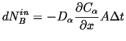
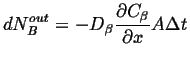
Diffusion with Moving Interfaces
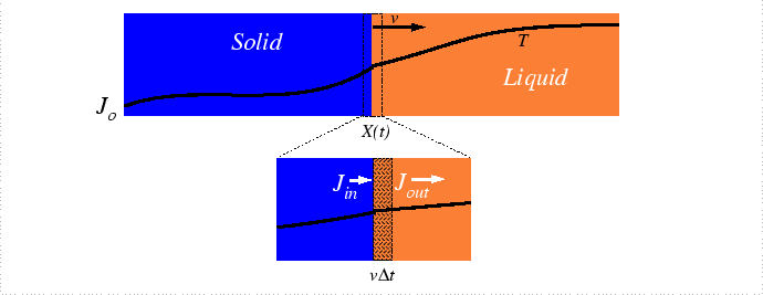
The methods for solving the diffusion equation were presented for cases of fixed boundary conditions. However, there many examples of kinetic processes in materials where boundaries (e.g. interfaces, phase boundaries) move in response or because of diffusion. Below, methods to treat such problems will be shown to be straightforward extensions of the diffusion equation-the additional physics is a conservation principle relating the velocity of the moving interface the rate at which a conserved quantity is consumed per unit area of the interface. While exact solutions are difficult to obtain, a few general results and approximations can be obtained and applied to materials processes.
The analysis of the moving interface problem originates with Stefan who was developing a model for the rate of melting of the polar ice-caps and icebergs. This problem remains as one of the biggest alloy solidification problems. Heat must be conducted from the oceans to the melting interface to to provide the latent heat of melting and salt must be supplied as well since the equilibrium concentrations salt in the liquid and solid differ.
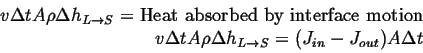
Interface Motion due to Heat Absorption at the Interface
To simplify the analysis of the problem, consider the heat-flux problem independently; specifically, consider freezing a liquid-solid mixture by extraction of heat:
 |
Assuming density, ![]() , is same in each phase, and equating the
volume swept out with heat required for the phase change:
, is same in each phase, and equating the
volume swept out with heat required for the phase change:
 |
(26-1) |
It is probably wise to check for wayward minus signs.
Consider the usual case,
![]() ,
and suppose the thermal diffusivity in the solid phase is zero (i.e. all
heat is
absorbed by the interface and supplied by the liquid reservoir); does the
velocity of
the interface have the expected sign?
,
and suppose the thermal diffusivity in the solid phase is zero (i.e. all
heat is
absorbed by the interface and supplied by the liquid reservoir); does the
velocity of
the interface have the expected sign?
Therefore the thermal diffusion equations become:
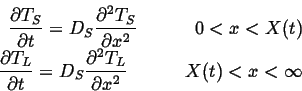 |
(26-3) |
| (26-4) |
 |
(26-5) |
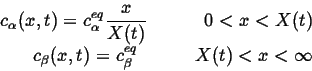
Mass Diffusion in an Alloy
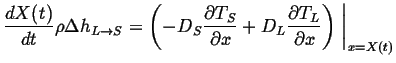
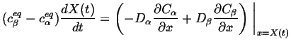
The Stefan condition relates the velocity of the interface to the ``jump'' in the density of an extensive quantity. For the case of heat above, that quantity was the enthalpy density. Next, the diffusion of chemical species will be coupled to the jump in alloy composition (amount/volume) at a moving interface--an analogous Stefan condition results.
Consider a diffusion couple between two alloys at different compositions for a system with multiple phases in equilibrium at a given temperature.
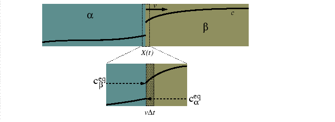 |
The mass balance at the moving interface is related to the phase diagram:
| (26-6) |
This must be balance by the amount going in:
 |
(26-7) |
 |
(26-8) |
Therefore, the Stefan condition is:
 |
(26-9) |
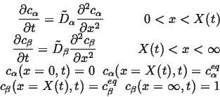
Simple Stefan Example
A limiting case for the mass diffusion case is developed below; the
result that the interface grows as ![]() is derived.
This result, as shown in the textbook, is a general one for
the Stefan problem with uniform diffusivity in each phase. Therefore,
this result is applicable to materials processes where material must
diffuse through a growing phase towards an interface where is can react
and form new material--such as oxidation of a surface.
is derived.
This result, as shown in the textbook, is a general one for
the Stefan problem with uniform diffusivity in each phase. Therefore,
this result is applicable to materials processes where material must
diffuse through a growing phase towards an interface where is can react
and form new material--such as oxidation of a surface.
The coupled diffusion equations are:
 |
(26-10) |
With the simplifying assumptions that
![]() and
a steady-state profile applies in
and
a steady-state profile applies in ![]() -phase, the concentration profiles
become:
-phase, the concentration profiles
become:
 |
(26-11) |
Incorporating this limiting case into the Stefan condition and integrating,
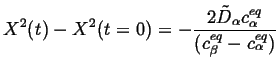 |
(26-12) |
Morphological Instabilities
A growth interface can undergo a morphological instability in cases when the driving force for growth (or transformation) is very large. The commonly observed example is that of a snowflake--which is a beautiful structure, but from simple considerations may appear to have much more surface energy than one might expect. In fact, the surface energy `competes' with the driving force for transformation--as the driving force increases, the amount of `extra' surface of the growth shape increases. On the other hand, if surface tension is very large compared to the volumetric driving force then the tendency for an interface to become unstable is decreases.
Instability of a Pure Liquid-Solid Interface
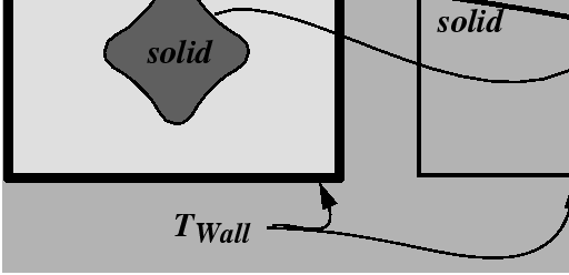
Consider the solidification of a pure liquid above its melting point by removing heat through a walls which are kept at a fixed temperature.
In this case, solidification begins at the walls and the solidification interface moves towards the center of the container at a rate which is dictated by how fast the latent heat of solidification can be conducted through the freshly grown solid phase and out through the walls. In this case, the interface is completely stable and the interface moves stably until all the liquid disappears.
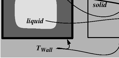
Now consider the solidification of a pure liquid which has been carefully supercooled below its melting point with no nucleation. If the solid phase is nucleated by a seed at the center of the container, then solidification proceeds as heat is conducted to the supercooled liquid and through the container walls.
If effects of gravity are eliminated, then such an experiment can be carried out with only thermal diffusion through the liquid phase and no convection. In this case, the interface is unstable and any small undulations in the surface can grow into dendrites.
The essential difference between Figure 26-4 and Figure 26-5 is that in the unstable case the new phase is growing into an unstable phase. The basic idea can be described in fairly simple terms. The supercooled liquid conducts heat which is generated by solidification; when a small protuberance forms at the interface, it pokes into liquid at a slightly lower temperature which can more efficiently conduct heat and therefore the protuberance continues to grow.
Alloy Solidification
A typical casting microstructure has a morphological instability:
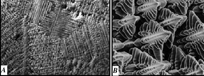 |
This is a puzzle: The morphological instability occurs for the case illustrated in Fig. 26-4--which is the case that was argued to be stable.
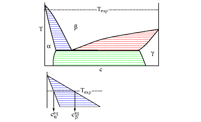
Constitutional Supercooling
The puzzle is solved by showing that the liquid near the growing interface is made unstable by composition variations due to the limited rate of mass diffusion. In this case, the instability is due to composition and not temperature.
The analogy between the thermal instability of a pure substance and the instability of alloy at constant temperature can be understood by referring to an isothermal line in a binary phase diagram.
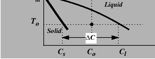 |
For a solid growing into a liquid phase, the advancing solid must reject solute into the liquid phase. The rate of advance is limited by the rate at which rejected solute can be diffused away, just as in the thermal case where interface motion is limited by the rate at which heat is diffused away.
Suppose that a material with a uniform composition, ![]() in
Fig. 26-7, is uniformly quenched into the
two-phase region.
The liquid is effectively under-cooled; such a system is
called constitutionally under-cooled.
Thus, a solidification front which starts from the edges of the
container will become unstable for the same reasons that the
front in
26-5
is unstable.
in
Fig. 26-7, is uniformly quenched into the
two-phase region.
The liquid is effectively under-cooled; such a system is
called constitutionally under-cooled.
Thus, a solidification front which starts from the edges of the
container will become unstable for the same reasons that the
front in
26-5
is unstable.
Mullins-Sekerka Instability
Both the constitutional supercooling and the thermal undercooling interfaces were analyzed by Mullins and Sekerka. They were able to determine a relationship between the wavelength of the instability, the surface tension, the transport coefficients, and the driving forces.
The analysis begins by introducing a dimensionless variable for temperature in one case and composition in the other:
 |
(26-13) |
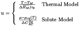
The interface condition is related to the curvature through the Gibbs-Thompson effect:
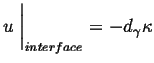 |
(26-14) |
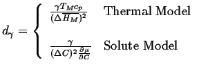 |
(26-15) |
This can be inserted into a set of moving interface diffusion equations and the stability of the interface can be evaluated by perturbation analysis.
All perturbation wavelengths greater that
![]() can grow:
can grow:
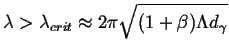 |
(26-16) |
The fastest growing wavelength is given by
| (26-17) |