| Conjugate Forces, Fluxes and Empirical Flux Laws for Unconstrained Components | ||||
| Quantity | Flux | Conjugate Force | Empirical Flux Law | |
| Heat |
|
Fourier's |
|
|
| Mass |
|
|
Modified1Fick's form |
|
| Charge |
|
|
Ohm's |
|
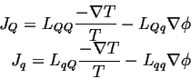
Entropy Production for Simple Cases
If heat is the only quantity that is flowing:
 |
(03-1) |
If diffusion is the only operating process:
| (03-2) |
In general, the entropy production is the sum of all operating fluxes dotted into (minus) the gradient of the associated potential.2
Generalized Coupling for the Near-Equilibrium Case
Let
![]() represent the generalized driving
forces for a system near equilibrium.
A system near equilibrium is one where the driving forces are all small, therefore
we can expand the fluxes in terms of these small driving forces:
represent the generalized driving
forces for a system near equilibrium.
A system near equilibrium is one where the driving forces are all small, therefore
we can expand the fluxes in terms of these small driving forces:
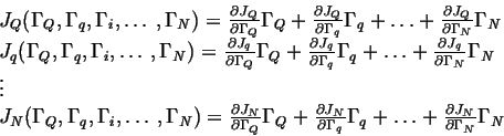 |
(03-6) |
or,
It is important to remember the origin of the ![]() .
They are derived as the linear coefficients of driving forces around the
equilibrium state-i.e. the case of condition of small driving forces.
Remember that if a function,
.
They are derived as the linear coefficients of driving forces around the
equilibrium state-i.e. the case of condition of small driving forces.
Remember that if a function, ![]() is expanded around a particular
point up to linear terms:
is expanded around a particular
point up to linear terms:
 |
(03-8) |
The values of the linear terms are functions of the point about which they
are expanded (
![]() ), so in the
expansion in Eq. 3-7, the linear coefficients
), so in the
expansion in Eq. 3-7, the linear coefficients
![]() are
also functions of the particular equilibrium state about which the
system is expanded. In other words, we should expect the
are
also functions of the particular equilibrium state about which the
system is expanded. In other words, we should expect the
![]() to be functions of temperature, equilibrium chemical potential, pressure, etc.
to be functions of temperature, equilibrium chemical potential, pressure, etc.
The entropy production for the near-equilibrium case is given by:
| (03-9) |
Because the term on the right hand side must be positive
definite and because each term is real, it is
necessary that the matrix
![]() is
symmetric;
this is
is
symmetric;
this is ![]() :
:
| (03-10) |
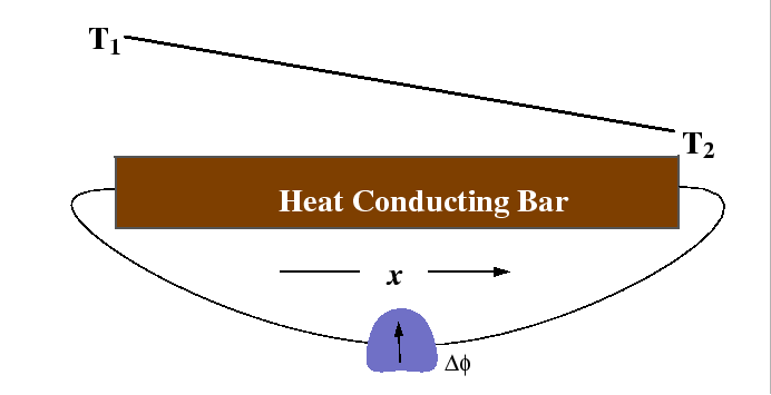
Example: Thermal and Ionic Conducting Bar
Consider heat transport in a bar that can conduct both heat and electricity via ionic conductivity:
Suppose there is no electric current (perfect voltmeter), then
 |
(03-12) |
 |
(03-13) |
A set of such physical experiments is considered below.
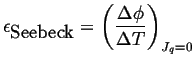
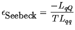
Seebeck, Peltier Effects and Thomson's Second Relation
Consider the following experimental set-up:
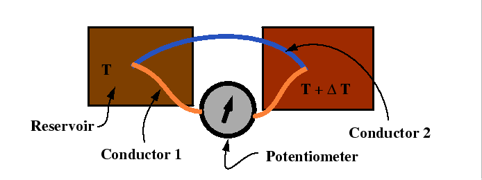 |
In the Seebeck a potential difference is set up in response to the flow of heat between two reservoirs.
The thermoelectric power is a relation between the potential difference and the temperature difference:
 |
(03-14) |
 |
(03-15) |
For the Peltier effect, the experimental set up is illustrated by:
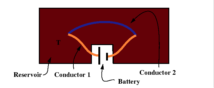 |
The Peltier coefficient is related to the ratio of the heat flux to the electric current:
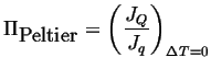 |
(03-16) |
Using equations 3-11, the Peltier coefficient can be calculated in terms of the Onsager coefficients:
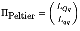 |
(03-17) |
If Onsager's symmetry relation holds (
![]() ),
then there must be a relation between the Peltier
and Seebeck coefficients:
),
then there must be a relation between the Peltier
and Seebeck coefficients:
| (03-18) |
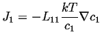
One Independent Mobile Species
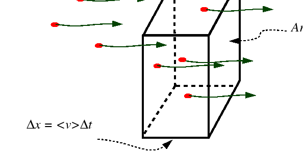
Consider the case of one chemical species that can diffuse independently of all the others, such as an interstitial carbon atom diffusing in BCC iron, or the case where a gaseous species is diffusing through a quiescent gas mixture.
Suppose that the only driving force is the gradient in chemical potential of the interstitial species, then
| (03-19) |
The chemical potential can be related to local concentration through
the activity coefficient ![]() :
:
| (03-20) |
Therefore,
![]() can be related to
can be related to
![]() :
:
For the ideal case, the activity coefficient is independent of concentration, so
 |
(03-21) |
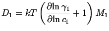
For the case of a non-ideal solution:
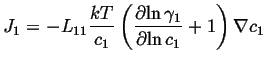 |
(03-22) |
If this is compared to the most simple version of Fick's first law,
![]() ,
, ![]() is called the intrinsic diffusivity and it
is related to the Onsager coefficient as:
is called the intrinsic diffusivity and it
is related to the Onsager coefficient as:
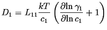 |
(03-23) |
The atomic mobility be defined by the the Einstein relation between the
average drift velocity and the driving force,
![]() .
.
 |
| (03-24) |
| (03-25) |
| (03-26) |
 |
(03-27) |
If the solution is ideal--as in the case of mixture of
radioisotopes of an otherwise identical atomic species--then the
diffusivity is called the self-diffusivity ![]() and since
the activity coefficient is constant:
and since
the activity coefficient is constant:
| (03-28) |