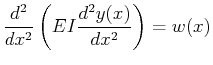
Link to Current (updated) notes

Fourth Order ODEs, Elastic Beams

Another linear ODE that has important applications in materials science is that for the deflection of a beam. The beam deflection $y(x)$ is a linear fourth-order ODE:

$$\ensuremath{\frac{d^2{}}{d{x}^2}} \left( EI \ensuremath{\frac{d^2{y(x)}}{d{x}^2}}\right) = w(x)$$ (21-17)

where $w(x)$ is the load density (force per unit length of beam), $E$ is Young's modulus of elasticity for the beam, and $I$ is the moment of inertia of the cross section of the beam:

$$I = \int_{\text{A}_{\times-sect}} y^2 dA$$ (21-18)

is the second-moment of the distribution of heights across the area.

If the moment of inertia and the Young's modulus do not depend on the position in the beam (the case for a uniform beam of homogeneous material), then the beam equation becomes:

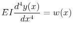
$$E I \ensuremath{\frac{d^{4}{y(x)}}{d{x}^{4}}} = w(x)$$ (21-19)

The homogeneous solution can be obtained by inspection--it is a general cubic equation $y_{homog}(x) = C_0 + C_1 x + C_2 x^2 + C_3 x^3$ which has the four constants that are expected from a fourth-order ODE.

The particular solution can be obtained by integrating $w(x)$ four times--if the constants of integration are included then the particular solution naturally contains the homogeneous solution.

The load density can be discontinuous or it can contain Dirac-delta functions $F_o \delta(x-x_o)$ representing a point load $F_o$ applied at $x=x_o$ .

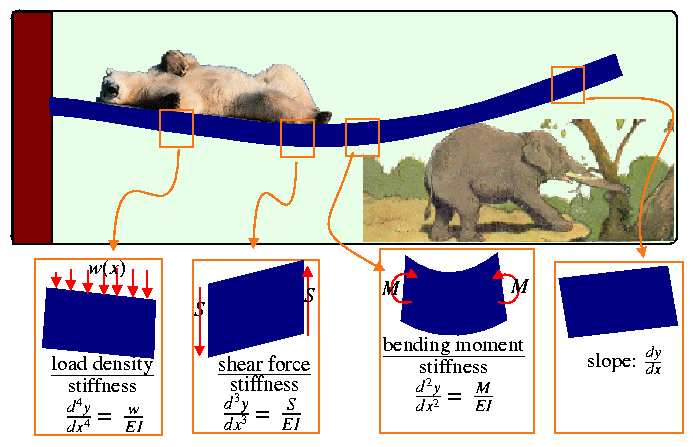
It remains to determine the constants from boundary conditions. The boundary conditions can be determined because each derivative of $y(x)$ has a specific meaning as illustrated in Fig. 21-2.

Figure 21-2: The shape of a loaded beam is determined by the loads applied over its length and its boundary conditions. The beam curvature is related to the local moment (imagine two handles rotated in opposite directions on a free beam) divided by the effective beam stiffness. Shear forces are related to the rate of change of moment along the beam.
(Polar Bear Photo Art Wolfe The Zone Network
http://classic.mountainzone.com/climbing/greenland/graphics/polar-bear.html )

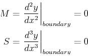
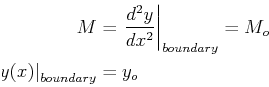
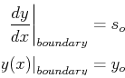
There are common loading conditions that determine boundary conditions:

Free

No applied moments or applied shearing force:

$$\begin{split} M & = \left.\ensuremath{\frac{d^2{y}}{d{x}^2}}... ...rac{d^{3}{y}}{d{x}^{3}}}\right\vert _{boundary} = 0 \end{split}$$

Point Loaded

local applied moment, displacement specified.

$$\begin{split} M & = \left.\ensuremath{\frac{d^2{y}}{d{x}^2}}... ... = M_o\\ \left.y(x)\right\vert _{boundary} & = y_o \end{split}$$

Clamped

Displacement specified, slope specified

$$\begin{split} \left.\ensuremath{\frac{d{y}}{d{x}}}\right\ver... ... = s_o\\ \left.y(x)\right\vert _{boundary} & = y_o \end{split}$$

MATHEMATICA$^{\text{\scriptsize {\textregistered }}}$ Example

(notebook Lecture-23)

(html Lecture-23)

(xml+mathml Lecture-23)

Visualizing beam deflections