Link to Current (updated) notes

Differential Equations: Introduction

Ordinary differential equations are relations between a function of a single variable, its derivatives, and the variable:

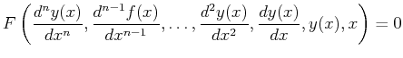$$F\left(\ensuremath{\frac{d^{n}{y(x)}}{d{x}^{n}}}, \ensuremath{\fr... ...\frac{d^2{y(x)}}{d{x}^2}},\ensuremath{\frac{d{y(x)}}{d{x}}}, y(x), x\right) = 0$$ (19-1)

A first-order Ordinary Differential Equation (ODE) has only first derivatives of a function.

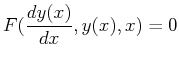$$F(\ensuremath{\frac{d{y(x)}}{d{x}}}, y(x), x) = 0$$ (19-2)

A second-order ODE has second and possibly first derivatives.

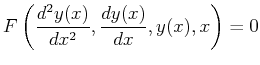$$F\left(\ensuremath{\frac{d^2{y(x)}}{d{x}^2}},\ensuremath{\frac{d{y(x)}}{d{x}}}, y(x), x\right) = 0$$ (19-3)

For example, the one-dimensional time-independent Shrödinger equation,

$$\begin{split} & -\frac{\hbar}{2m} \frac{d^2 \psi(x)}{dx^2} ... ...^2 \psi(x)}{dx^2} + U(x) \psi(x) - E \psi(x) = 0\\ \end{split}$$

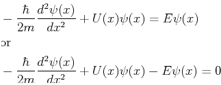
is a second-order ordinary differential equation that specifies a relation between the wave function, $\psi(x)$ , its derivatives, and a spatially dependent function $U(x)$ .

Differential equations result from physical models of anything that varies--whether in space, in time, in value, in cost, in color, etc. For example, differential equations exist for modeling quantities such as: volume, pressure, temperature, density, composition, charge density, magnetization, fracture strength, dislocation density, chemical potential, ionic concentration, refractive index, entropy, stress, etc. That is, almost all models for physical quantities are formulated with a differential equation.

The following example illustrates how some first-order equations arise:

MATHEMATICA$^{\text{\scriptsize {\textregistered }}}$ Example

(notebook Lecture-19)

(html Lecture-19)

(xml+mathml Lecture-19)

Iteration: First-Order Sequences

Consider a function that changes according to its current size-that is, at a subsequent iteration, the function grows or shrinks according to how large it is currently.

$$F_{i+1} = F_{i} + \alpha F_{i}$$

which is equivalent to

$$F_{i} = F_{i-1} + \alpha F_{i-1}$$

MATHEMATICA$^{\text{\scriptsize {\textregistered }}}$ Example

(notebook Lecture-19)

(html Lecture-19)

(xml+mathml Lecture-19)

First-Order Finite Differences

The example above is not terribly useful because the change at each increment is an integer and the function only has values for integers. To generalize, a forward difference can be added that allows the variable of the function to ``go forward'' at an arbitrarily small increment, $\delta$ .

If the rate of change of $y$ , is a function $f(y)$ of the current value, then,

$$y_{i+1} = y_i + \delta f(y_i)$$

or

$$y(x=(i+1)\delta)) = y(x=i \delta) + \delta f(y(x=i \delta))$$

where $x$ plays the role of an `indexed grid' with small separations $\delta$ .

MATHEMATICA$^{\text{\scriptsize {\textregistered }}}$ Example

(notebook Lecture-19)

(html Lecture-19)

(xml+mathml Lecture-19)

First-Order Operators

The forward-difference equation considered above relates the next iteration, $y_{i+1}$ to the current value $y_i$ . Only $y_i$ appear on the right-hand-side of the equation--the right-hand-side can be thought of an ``Operation'' on $y$ that pushes it to the next iteration, i.e.,

$$y_{i+1} = \mathcal{F}(y_i)$$

In this way, the $n^{th}$ iteration is determined from the initial value with

$$y_n = {\mathcal{F}}^n(y_0)$$