Perhaps the most straightforward of the higher-dimensional integrations (e.g., vector function along a curve, vector function on a surface) is a scalar function over a domain such as, a rectangular block in two dimensions, or a block in three dimensions. In each case, the integration over a dimension is uncoupled from the others and the problem reduces to pedestrian integration along a coordinate axis.
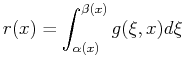
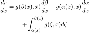
Sometimes difficulty arises when the domain of integration is not so
easily described; in these cases, the limits of integration
become functions of another integration variable.
While specifying the limits of integration requires a bit
of attention, the only thing that makes these cases difficult is
that the integrals become tedious and lengthy.
MATHEMATICA![]() removes some of this burden.
removes some of this burden.
A short review of various ways in which a function's variable can appear in an integral follows:
|
The Integral
|
Its Derivative
|
|
|
Function
of limits |
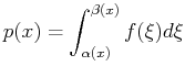
|
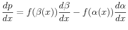
|
|
Function
of integrand |
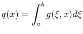
|
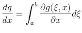
|
|
Function
of both |
|
|
| Extra Information and Notes
Potentially interesting but currently unnecessary |
||||||||
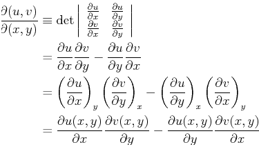
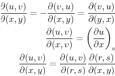
| Changing of variables is a topic in multivariable calculus that
often causes difficulty in classical thermodynamics.
This is an extract of my notes on thermodynamics: http://pruffle.mit.edu/3.00/ Alternative forms of differential relations can be derived by changing variables. To change variables, a useful scheme using Jacobians can be employed:
For example, the heat capacity at constant volume is:
Using the Maxwell relation,
which demonstrates that |
|
MATHEMATICA |
| (notebook Lecture-14) |
| (html Lecture-14) |
| (xml+mathml Lecture-14) |
| Potential near a Charged and Shaped Surface Patch
Example calculation of the spatially-dependent energy of a unit point charge
in the vicinity of a charged planar region having the shape of an equilateral
triangle.
The energy of a point charge
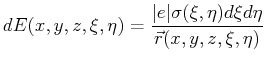
for a patch with uniform charge,
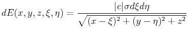
For an equilateral triangle with sides of length one and center at the origin, the vertices can be located at
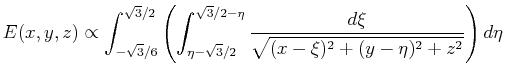
MATHEMATICA Integrate[1/r[x,y,z], {x,a,b}, {y,f[x],g[x]}, {z,p[x,y],q[x,y]}] would integrate over |
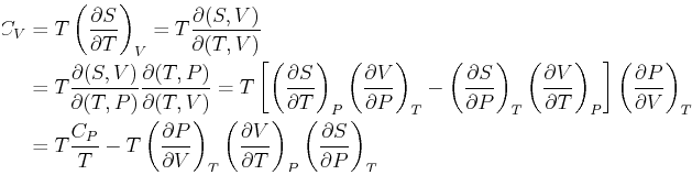
![$\displaystyle C_P - C_V = -T \frac{ [ \ensuremath{ \left( \frac{\partial{V}}{\p...
...P} } ]^2 }{ \ensuremath{ \left( \frac{\partial{V}}{\partial{P}} \right)_{T} } }$](img57.png)