Last time: Particle coarsening.--II

Elements of mean-field theory for DCC

• Growth rate of a particular particle of radius $R_{i}$ from supersaturated solution

  
  

• The particle-size distribution function $f(r,t)$ and its associated continuity equation

  
  

• Key result (1): Steady-state (normalized) particle-size distribution function

  
  

• Key result (2): Functional dependence of mean particle size $<R>$ on time

  
  

Complications of real systems

• Nonzero volume fraction; particle-particle interactions

  
  

• Coherency stresses

  
  

• Applied stresses

  
  

Experimental study of coarsening in semi-solid Pb-Sn alloys (Hardy and Voorhees 1988

Today: Phase Transformations: Overview

Metastability, instability, and mechanisms

First-order and second-order transitions

Free energy functions; conserved and nonconserved variables

Spinodal decomposition--I.

• Diffusion within the spinodal

3.21 Spring 2001: Lecture 27

Phase Transformations: Overview

Metastability, instability, and mechanisms

A phase transformation can occur when a system has an accessible state of lower free energy. The mechanism of the transformation is critically dependent on whether the starting state is metastable or unstable.

An unstable system can transform by making changes that are small in degree but large in extent. Such situations lead to mechanisms that are called continuous transformations. The main categories of continuous transformations in materials are spinodal decomposition and continuous ordering.

A metastable system can transform by making changes that are large in degree but small in extent. Such situations require nucleation of the new phase. After nucleation takes place, a new particle can grow until it either impinges with another particle, or supersaturation of the surrounding material is depleted.

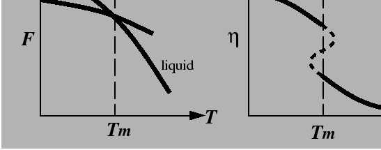
First-order and second-order transitions

Ehrenfest proposed a useful scheme for classification of phase transformations based on discontinuities in derivatives of the free energy function $F$ that are characteristic of the transformation. Simply put, the order or a phase transformation is the lowest order of the derivative of $F$ that shows a discontinuity.

Examples: melting; ordering in $\beta$ brass

Decomposition into Phases: Conserved Fields

Figure 27-1: Decomposition requires long-rang diffusion. Such a transformation requires flux of a conserved field, like composition $c(x)$, which has an integral that is conserved for a closed system.

Order-Disorder: Nonconserved Fields

Figure 27-2: The phase change does not require long-rang diffusion. Such a transformation involves local changes in some field, like the order parameter $\eta (x)$, which is not conserved for a closed system.

Order Parameters and Phase Transformations

Consider a simple one component phase transformation:

Figure 27-3: Representations of simple thermodynamic constructions for phase transformations.

We can express the transformation near the transition as a Landau expansion

$$F(T,\eta) = a_0(T) + a_1(T) \eta + a_2(T) \eta^2 + \ldots$$ (27-1)

where $\eta$ might be some measure of a ``hidden parameter'' such as the diffuseness of a peak in the atomic radial-distribution function.

The equilibrium value of $F$ is given by

$$\frac{\partial F}{\partial \eta} = 0$$ (27-2)

so the equilibrium free energy is given by $F(T, \eta(T))$. Whether the phase transition is first-order or second-order will depend on the relative magnitude of the coefficients of the Landau expansion.

We will use functions like $F(T,\eta)$ to follow evolution towards equilibrium values $F(T, \eta(T))$.

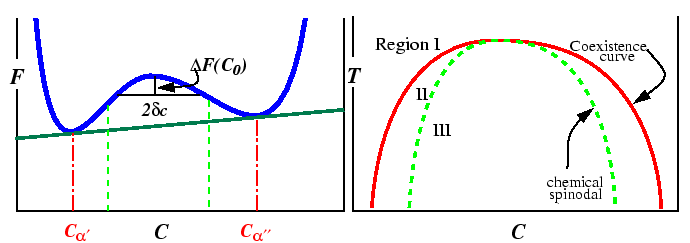
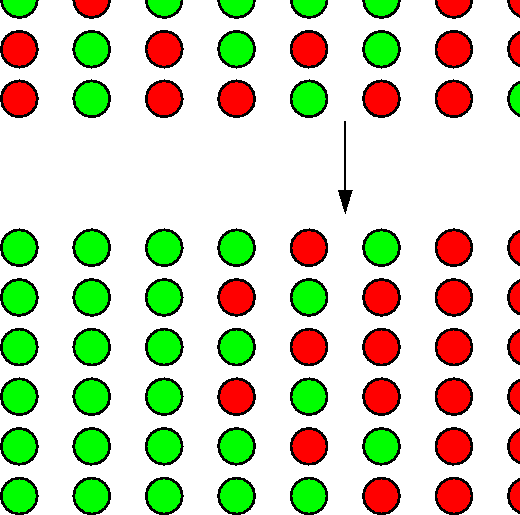
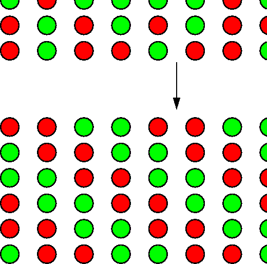
Spinodal decomposition

The chemical spinodal and "uphill diffusion"

Recall that

$$\tilde{D} = (c D_A^* + (1-c)D_B^*) ( 1 + \ensuremath{\frac{\parti... ...A^* + (1-c)D_B^*) \frac{c}{RT} \ensuremath{\frac{\partial{\mu_A}}{\partial{c}}}$$ (27-3)

Note that since, $\mu \equiv \ensuremath{\frac{\partial{\bar{F}}}{\partial{c}}}$, that the diffusivity has the same sign as the second derivative of the free energy:

$$\tilde{D} \propto \ensuremath{\frac{\partial^2{\bar{F}}}{\partial{c}^2}}$$ (27-4)

Consider the following free-energy curve and resulting phase diagram:

Figure 27-4: Prototype free-energy construction and resulting phase diagram with a spinodal region.

In region III, $\tilde{D} < 0$, how does the diffusion equation behave when $\tilde{D} < 0$? Recall that for initial conditions $c(x,t=0) = A(t=0) \sin \frac{2 pi x}{\lambda}$ the diffusion equation has solution:

$$A(t) = A(0) e^{- \tilde{D} (\frac{2 pi x}{\lambda})^2 t}$$ (27-5)

This will be very badly behaved for small wavelengths and give no end of trouble. It is ill-posed.

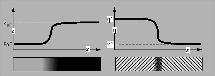
Gradient Energy

How to fix this problem and calculate a governing equation inside the spinodal region?

Consider the following profile or variation in field:

Figure 27-5: Introduction of the diffuse interface.

What kind of penalties can be imposed that ``mimic'' surface energy?

Should the penalty depend on the whether the field is increasing left-to-right or increasing right-to-left?

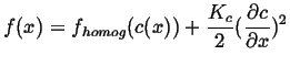
For inhomogenous fields, expand the free energy about its homogenous value:

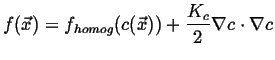$$f(\vec{x}) = f_{homog} (c(\vec{x})) + \frac{K_c}{2} \ensuremath{\nabla}c \cdot \ensuremath{\nabla}c$$ (27-6)

$K$ is the gradient energy coefficient, it introduces surface energy into the free energy and will ``regularize'' the diffusion equation within (and applies outside as well) the spinodal.

For one-dimensional variations, the free energy density is:

$$f(x) = f_{homog} (c(x)) + \frac{K_c}{2} (\ensuremath{\frac{\partial{c}}{\partial{x}}})^2$$ (27-7)

Theory of diffuse interfaces