Complex Valued Roots to Polynomial Equations

Complex numbers frequently appear in the solution of roots to polynomial equations:

The next statement produces a list of the complex solutions of the polynomial:

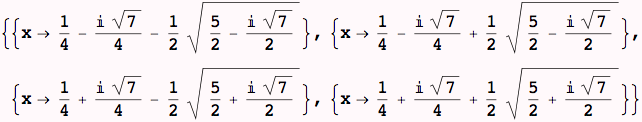
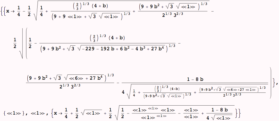
Generalize the above to a family of solutions: find b such that imaginary part of the solution vanishes

This will give a list of rules that can be used to find solutions;as "b" is unspecified the rules depend on the symbol "b"
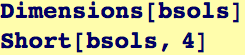
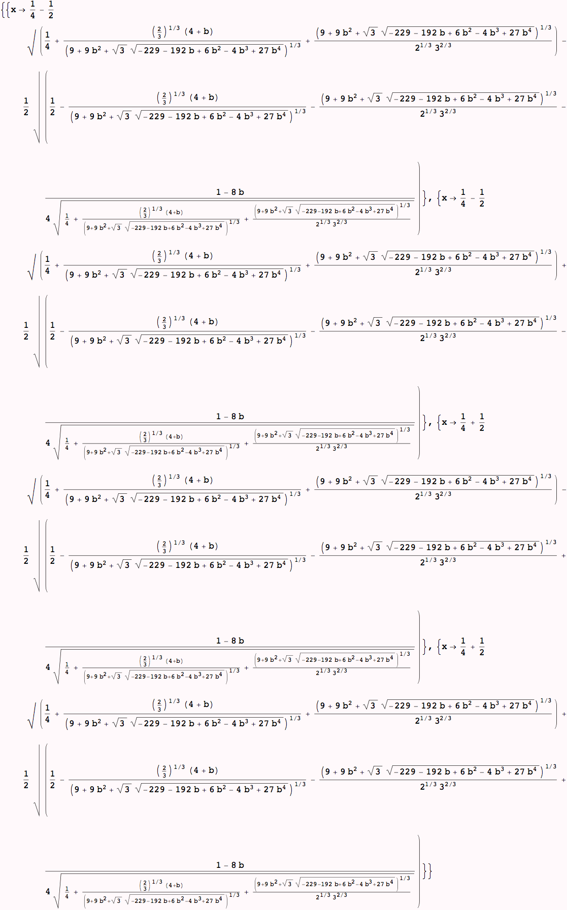
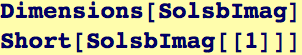
Because it is a long set of rules and hard to follow, let's look at the form of bsols:
Short produces a very abbreviated form of the solution… in this case limited to 3 lines by the optional parameter.

So we see that bsols is a list of length 4 of list containing one rule. (Solutions to equations are always this way, it is a list of the number of solutions, each member being a rule for each variable that is solved for...)

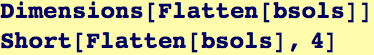
In our case of one variable, the extra layer of lists is not terribly useful, one way to get rid of the extra layers is to use Flatten:

In the next command, we produce a list of values (not of rules, because we have taken x and applied every rule in bsols to it... These values are the imaginary parts of the solutions x that make the polynomial vanish (and a function of b, because it hasn't been specified yet)

**Note,on some machines this next command will take a while to finish**

And likewise for the real parts of x that solve the polynomial equation

**Note,on some machines this next command will take a while to finish**

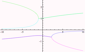
This plot works as follows, for each member in the list, plot the result of replacing b with values  between -10, 10. So the following should be  a plot of the imaginary values of x as a function of b.

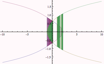
There are a few problems that make it difficult to interpret the graph---one is the numerical noise that makes the solutions jump back and forth; second, because all the colors are the same,  it is not clear which values of x belong to the same solution.  

Let's first try to make each member of the list (remember, there are 4 because it is a fourth-order polynomial and because Dimensions[imb] told us so...

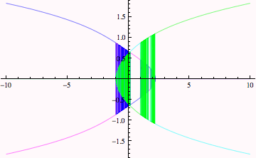
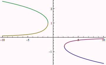
The plot above is a little better, it looks like the blue curve comes in from the northeast and then then its imaginary part vanishes at a critical values of b (around -0.5), the cyan curve is probably the minus values of the blue curve... and the same thing for yellow and green.  It is much easier to see the branches of solutions for the real parts below.

But here, because the lines are the same thickness, we don't know if the cyan and blue curves just "stop." Let's find out by also adjusting their thickness.

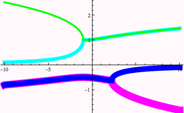
It is pretty clear that the parameter b is behaving like a "pitchfork" bifurcation---there is one value of x upto a critical value of b, where x splits into two solutions.  This is a picture of two isolated pictchforks.

As of Mathematica 6, the argument to Plot doesn't have to evaluate to a real number. As of Mathematica 6, Plot will skip values at which the functions don't evaluate to a real number.  Below, we can see that there are two real solutions for b < -1 and again for a little more than b > 2.

Created by Wolfram Mathematica 6.0  (07 September 2007)