Basis and Orthogonal Functions
This is a generalization of the Fourier series. The orthogonality of the trignometric functions
(i.e.,  Sin[2 π n x] Sin[2 π m x]dx =
 |
if n=m |
| 0 |
if n≠m |
)
was the key to the ``trick'' that permitted calculation of the Fourier coefficients.
This is a generalization of dot or scalar vector product, but for functions. The norm that is defined above for the trignometric functions is fairly simple, it is the l2-norm:
f(x) • g(x) ≡ ∫ f(x) g(x) dx (l2-norm)
However, there can be many other types of norms, for instance a Gaussian weighted l2-norm
f(x) • g(x) ≡ ∫ f(x) g(x)  dx (Gaussian weighted l2-norm)
and many many others.
Both the norm and the domain of integration must be defined.
To represent a function in terms of a sum of basis functions with coefficients, a orthogonality relation must be obtained for the basis functions.
We will do a few examples of orthogonality relations, the coefficients can be found as a straightforward extension of the Fourier method.
Establish by example the orthogonality relations for the Lengendre Polynomials
In[115]:=
![Table[Integrate[LegendreP[i, x] LegendreP[5, x], {x, -1, 1}], {i, -10, 10}]](HTMLFiles/Lecture-27_4.gif)
Out[115]=
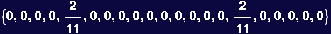
Calculate the norm as a function of the order of the Legendre polynomial
In[116]:=
![Table[Integrate[LegendreP[i, x] LegendreP[i, x], {x, -1, 1}], {i, 0, 15}]](HTMLFiles/Lecture-27_6.gif)
Out[116]=

Make a guess at what the norm looks like
In[117]:=
![Table[2/(2 i + 1), {i, 0, 15}]](HTMLFiles/Lecture-27_8.gif)
Out[117]=

The orthogonality relation is plausibly:  LegendreP[i,x] LegendreP[j,x]dx =
 |
if | i|=|j| |
| 0 |
if |i |≠|j| |
In fact, this is correct
Representation of a function in terms of the Legendre basis
This demonstrates how to take a specific set (basis) of orthogonal functions and represent an arbitrary function in terms of an infinite sum of terms involving the basis functions, each with its own coefficient. This is a direct analog to what we did with Fourier series.
A function to calculate the coefficients
In[118]:=
![LegendreCoefficient[f_, i_] := (2 i + 1)/2Integrate[f[x] LegendreP[i, x], {x, -1, 1}]](HTMLFiles/Lecture-27_12.gif)
Use Legendre functions to represent the function 
This is an example function:
In[119]:=
![AFunc[x_] := Exp[-x^2]](HTMLFiles/Lecture-27_14.gif)
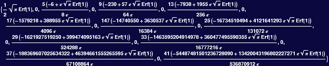
Calculate the first twenty coefficients
In[120]:=
![Lcofs = Table[LegendreCoefficient[AFunc, i], {i, 0, 20}]](HTMLFiles/Lecture-27_15.gif)
Out[120]=
Construct a vector of the eigenfunctions
In[121]:=
![Lfuncs = Table[LegendreP[i, x], {i, 0, 20}] ;](HTMLFiles/Lecture-27_17.gif)

Visualize the approximation of the first twenty terms
In[122]:=
![Plot[{Lcofs . Lfuncs, Exp[-x^2]}, {x, -1, 1}, PlotStyle→ {{Hue[0], Thickness[0.01]}, {Hue[0.66], Thickness[0.005]}}]](HTMLFiles/Lecture-27_19.gif)
![[Graphics:HTMLFiles/Lecture-27_20.gif]](HTMLFiles/Lecture-27_20.gif)
Out[122]=

Try another function
In[123]:=
![AFunc[x_] := Sin[5x] Sin[(5 + 1/10) x]](HTMLFiles/Lecture-27_22.gif)
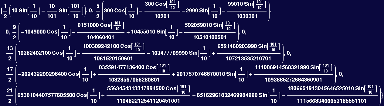
Coefficients out to 10 terms
In[124]:=
![Lcofs = Table[LegendreCoefficient[AFunc, i], {i, 0, 10}]](HTMLFiles/Lecture-27_23.gif)
Out[124]=
In[125]:=
![Lfuncs = Table[LegendreP[i, x], {i, 0, 10}] ;](HTMLFiles/Lecture-27_25.gif)
Visualize the approximation
In[126]:=
![Plot[{Lcofs . Lfuncs, AFunc[x]}, {x, -1, 1}, PlotStyle→ {{Hue[0], Thickness[0.01]}, {Hue[0.66], Thickness[0.005]}}]](HTMLFiles/Lecture-27_26.gif)
![[Graphics:HTMLFiles/Lecture-27_27.gif]](HTMLFiles/Lecture-27_27.gif)
Out[126]=