Phase Plane Analysis of Linear Differential Equations

Description of behavior from coefficients of linear expansion about fixed point

Write a set of function that predict the behavior of the system  = (

Note: This is a first-order ODE with constant coefficients. Its solution will be a sum of two exponential functions with the form . The characteristics of the system of two equations are determined by the eigenvalues and eigenvectors of the matrix of coefficients, as detailed by the analysis and examples presented below.

Note that the eigenvalues are either real or they are complex conjugates (i.e., the eigenvalues are the solutions to  the quadratic equation)

Here is a function to print out a warning if the eigenvalues are inconsistent with a real coefficient matrix:

In[54]:=

Here is a function that prints out information about stability based on the eigenvalues:

In[55]:=

Here is a function that prints out information about the type of fixed point:

In[56]:=

Here is a function that collects our other functions

In[57]:=

In[58]:=

In[59]:=

Here is a function that prints out information about the direction of the eigenvectors

In[60]:=

Here is a function that uses the coefficients to collect and print the physical information about the fixed point

In[61]:=

In[62]:=

Out[62]=

Visualization of Trajectories near Fixed Points in the Plane

Functions to find the solutions for input coefficients (first one for specified initial point; the second one for initial points picked randomly

In[63]:=

In[64]:=

In[65]:=

Out[65]=

Example of a plot for a single directory

In[66]:=

In[67]:=

Out[67]=

This is not terribly informative.  Construct a function that takes input and plots many paths with arrows that describe the trajectory.  Print out physical interpretations as well.  Supply an argument with  a default definition that indicates the number of trajectories to plot.

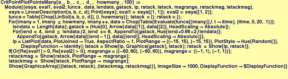
In[68]:=

In[69]:=

In this first example, the eigenvalues are real and negative, and the system of equations has a stable, attractive node. The eigenvectors are real and correspond to directions along which the system will evolve along a straight trajectory.

In[70]:=

Out[70]=

In this next example, the eigenvalues are real and positive, and the system of equations has an unstable node. The eigenvectors are real and correspond to directions along which the system will evolve along a straight trajectory.

In[71]:=

Out[71]=

In this next example, the eigenvalues are real and of opposite sign, and the system of equations has an unstable saddle point. The eigenvectors are real and correspond to directions along which the system will evolve along a straight trajectory.

In[72]:=

Out[72]=

In this next example, the eigenvalues are complex, with a positive real part, and the system of equations has an unstable circulation pattern. The eigenvectors are complex and and there are no directions along which the system will evolve along a straight trajectory.

In[73]:=

Out[73]=

In this next example, the eigenvalues are complex, with a negative real part, and the system of equations has an stable, attractive circulation pattern. The eigenvectors are complex and and there are no directions along which the system will evolve along a straight trajectory.

In[74]:=

Out[74]=

In this final example, the eigenvalues are pure imaginary, and the system of equations exhibit stable orbits around a fixed point. The eigenvectors are complex and and there are no directions along which the system will evolve along a straight trajectory.

In[75]:=

Out[75]=

Created by Mathematica  (November 21, 2005)