Lecture 21 MIT 3.016 (Fall 2005) © W. Craig Carter 2003-2005

Higher-Order Ordinary Differential Equations

Background: Another example of for Forward Differencing

Recall how we used forward finite differencing to simulate the behavior of a function that changed proportional to its current size in Lecture 19. Consider now a function that changes "how fast it changes" proportional to its current change and its current value--in other words its current acceleration is proportional to its velocity and to its size:

Let's work out how to find a finite differencing function:

This is the current change or approximation to velocity

CurrentChangePerDelta[F_, i_, Δ_] := (F[i + 1] - F[i])/Δ

This is the current change in change or approximation to acceleration

CurrentChangeinCurrentChangeperDelta[F_, i_, Δ_] := Simplify[(CurrentChangePerDelta[F, i + 1, Δ] - CurrentChangePerDelta[F, i, Δ])/Δ]

Our model is that the acceleration is proportional to size of the current function and its velocity, let these proportions be: -α and -β

α F[i] + (β (-F[i] + F[1 + i]))/Δ + (F[i] - 2 F[1 + i] + F[2 + i])/Δ^2 == 0

Solve this for the "latest" values

${F[2 + i] → -F[i] + β Δ F[i] - α Δ^2 F[i] + 2 F[1 + i] - β Δ F[1 + i]}$

Replace to find the form of the solution

${F[j] → -F[-2 + j] + β Δ F[-2 + j] - α Δ^2 F[-2 + j] + 2 F[-1 + j] - β Δ F[-1 + j]}$

Notice that this forward differnce needs TWO consectutive past values before it can calculate the current value, create a function to Appends the current value to a list by using the last two values:

The fact that TWO consecutive values are needed is not surprising. Because this iteration procedure is giving an approximation to the solution of a second-order ODE, we need to make a numerical approximation to a second derivative. THREE points—the two consecutive ones and the current one—are needed to do this. (If only two points were used, you could only compute the slope of the straight line connecting the points; if three points are used, a circle can be fit to the three points and the inverse of its radius gives the curvature.)

Define a function for specific parameters of the General case, and use it to generate a sequence of length 20

Visualize results (it takes about 45 seconds to visualize 20000 iterations)

[Graphics:HTMLFiles/Lecture-21_18.gif]

Change parameters for Growth Function:

[Graphics:HTMLFiles/Lecture-21_22.gif]

Second-Order Linear Homogeneous ODEs with Constant Coefficients, Analysis of the Solution Basis

Analysis of basis solutions to y'' + βy' + γy = 0 in terms of constant coefficients β and γ

First write a general expression for this homogeneous ODE:

$TheODE[function_, var_] := D[function[var], {var, 2}] + β D[function[var], var] + γ function[var]$

Guess a solution and substitute it into the left-hand side of the ODE:

This will be a solution when the resulting quadratic expression in λ is equal to 0:

${{λ→1/2 (-β - (β^2 - 4 γ)^(1/2))}, {λ→1/2 (-β + (β^2 - 4 γ)^(1/2))}}$

The two roots λ+ and λ+ are:

1/2 (-β + (β^2 - 4 γ)^(1/2))

1/2 (-β - (β^2 - 4 γ)^(1/2))

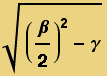
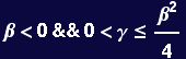
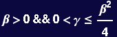
Assuming that β and γ are real, the solutions can be characterized by the roots of the quadratic equation. That is, our solution is known to be : the solution monotonically grows or shrinks in time if the roots are real-positive or real-negative. The condition that the roots are real is γ <

If the roots have an imaginary part, the solutions can oscillate. Whether the oscillation amplitudes grow or shrink depends on whether the real part of λ is positive or negative.

We now do some calculations to make an annotated map on the β–γ plane of solution scenarios for the λ values:

$ComplexReal = Plot[β^2/4, {β, -1, 1}, AxesLabel→ {"β", "γ"}]$

[Graphics:HTMLFiles/Lecture-21_39.gif]

$ComplexRealAnnote = Show[ComplexReal, Graphics[Text["Complex\nCongugate\nRoots", {0.25, 0.25}, {-1, 1}]], Graphics[Text["Real Roots", {0.75, 0.05}]]]$

[Graphics:HTMLFiles/Lecture-21_42.gif]

If the roots complex, then the sign of the real part is determined only by the sign of β; i.e., λ = ± ((β/2)^2 - γ)^(1/2)

[Graphics:HTMLFiles/Lecture-21_49.gif]

[Graphics:HTMLFiles/Lecture-21_52.gif]

Find the conditions where the real roots are positive and/or negative

β<0&&0<γ≤β^2/4

AnnoteMixedRealRoots = Show[MixedRealRoots, Graphics[Text[StyleForm["Mixed Real Roots", FontColor→Hue[.6]], {0.2, -0.1}, {-1, 0}]], DisplayFunction→$DisplayFunction]

[Graphics:HTMLFiles/Lecture-21_63.gif]

β>0&&0<γ≤β^2/4

[Graphics:HTMLFiles/Lecture-21_70.gif]

Determination of Specific Solution using Boundary Values

Second order ODEs require that two conditions be specified to generate a particular solution.

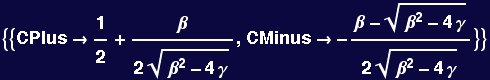
Example of y(0) = 0 and y(L)=1
The general solution will have the form:

$General :: spell1 : Possible spelling error: new symbol name \"CPlus\" is similar to existing symbol \"Plus\". More…$

$General :: spell1 : Possible spelling error: new symbol name \"CMinus\" is similar to existing symbol \"Minus\". More…$

Apply the two boundary conditions and solve the resulting equations for constants CPlus and CMinus:

Write the resulting solution:

(^(1/2 (L - x) (β + (β^2 - 4 γ)^(1/2))) (-1 + ^(x (β^2 - 4 γ)^(1/2))))/(-1 + ^(L (β^2 - 4 γ)^(1/2)))

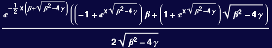
Second example with different form of boundary condition: y(0) = 1 and y'(0)=0

Now the constants CPlus and CMinus are found by solving:

${{CPlus→1/2 + β/(2 (β^2 - 4 γ)^(1/2)), CMinus→ -(β - (β^2 - 4 γ)^(1/2))/(2 (β^2 - 4 γ)^(1/2))}}$

And the new solution is:

Example of Higher-Order equation and Visualization of Solutions:
The Beam Equation

Visualizing Beam Deflections:

Set up the ODE solution (we will specify a unit beam stiffness) EI = 1

$BeamEquation[y_ , x_ , w_, BC1_ , BC2_] := DSolve[Flatten[{y''''[x] == w[x], BC1, BC2}], y[x], x]//Flatten$

Set up some typical boundary conditions:

$Clamped[y_ , x_ , position_, slope_] := {y[x] == position, y '[x] == slope}$

$PointLoad[y_, x_, position_, moment_] := {y[x] == position, y''[x] == moment}$

$FreeEnd[y_ , x_] := {y''[x] == 0, y'''[x] == 0}$

${y[x] →0. + 0. x - 0.15 x^2 + 0.05 x^3}$

Clamped Beam, loaded at the end

Plot[Evaluate[y[x]/.BeamEquation[y, x, noload, Clamped[y, 0, 0, 0], PointLoad[y, 1, -.25, 0]] ], {x, 0, 1}, PlotRange→ {-0.5, 0.5}, AspectRatio→1]

[Graphics:HTMLFiles/Lecture-21_94.gif]

Clamped Beam, Free end, unit applied load

Plot[Evaluate[y[x]/.BeamEquation[y, x, unitload, Clamped[y, 0, 0, 0], FreeEnd[y, 1]] ], {x, 0, 1}, PlotRange→ {-0.5, 0.5}, AspectRatio→1]

[Graphics:HTMLFiles/Lecture-21_98.gif]

Clamped Beam, Point load at end, Point load at Middle

Plot[Evaluate[y[x]/.BeamEquation[y, x, midload, Clamped[y, 0, 0, 0], PointLoad[y, 1, 0, 0]] ], {x, 0, 1}, PlotRange→ {-0.5, 0.5}, AspectRatio→1]

[Graphics:HTMLFiles/Lecture-21_102.gif]

Point Loaded on both ends, loaded in the middle as above

Plot[Evaluate[y[x]/.BeamEquation[y, x, midload, PointLoad[y, 0, 0, 0], PointLoad[y, 1, 0, 0]] ], {x, 0, 1}, PlotRange→ {-0.5, 0.5}, AspectRatio→1]

[Graphics:HTMLFiles/Lecture-21_106.gif]

Point Loaded on both ends, with linear distributed load positive at left and negative at right

Plot[Evaluate[y[x]/.BeamEquation[y, x, testload, PointLoad[y, 0, 0, 0], PointLoad[y, 1, 0, 0]] ], {x, 0, 1}, PlotRange→ {-0.5, 0.5}, AspectRatio→1]

[Graphics:HTMLFiles/Lecture-21_110.gif]

Clamped on both ends, with a "box" placed at x = 3/4

[Graphics:HTMLFiles/Lecture-21_114.gif]

Plot[Evaluate[y[x]/.BeamEquation[y, x, boxload, Clamped[y, 0, 0, 0], Clamped[y, 1, 0, 0]] ], {x, 0, 1}, PlotRange→ {-0.5, 0.5}, AspectRatio→1]

[Graphics:HTMLFiles/Lecture-21_117.gif]

Created by Mathematica (November 8, 2005)