Lecture 14 MIT 3.016 (Fall 2005) © W. Craig Carter 2003-2005

Integrals over a Curve, Multidimensional Integrals

We will look at two examples of path integrals of vector functions of position and examine their path dependence. The first integral has a non-zero curl (and so we know that it is not the gradient of some scalar potential)

Here is a vector function (xyz, xyz, xyz) for which the curl does not vanish anywhere

These are the conditions that the curl is zero:

There is only one point where this occurs:

Let's evaluate the integral of the vector potential ( ∮ •d ) for any curve that wraps around a cylinder of radius R with an axis that coincides with the z-axis
[Graphics:HTMLFiles/Lecture-14_12.gif]
Any curve that wraps around the cylinder can be parameritized as (x(t), y(t), z(t)) = (R cos(t), R sin(t), A (t)) where (t) = (t + 2π) and in particular (0) = (2π).
Therefore d= (-R sin(t), R cos(t), (t)) dt = (-y(t), x(t), A (t)) dt
The integrand for an integral of "VectorFunction" around such a curve is (written in terms of an arbitrary P(t):

The integral depends on the choice of P(t)

Let's introduce some specific periodic functions for P. Note how the value of the integral changes as the path changes:

1/4 Amp π Radius^2 (Amp + Radius)

-1/4 Amp π Radius^2 (Amp + Radius)

Amp Radius^2 ((3 Amp π)/2 - (8 π Radius)/9)

However, here is curious result which shows that some special paths can ``accidentally'' have zero integrals : let P(t) = cos(n t),

-(Amp Radius^2 (8 (-3 + n^2) Radius Sin[n π]^2 + n (-8 Radius + Amp (-9 + n^2) Cos[2 n π]) Sin[2 n π]))/(4 (9 - 10 n^2 + n^4))

[Graphics:HTMLFiles/Lecture-14_36.gif]

[Graphics:HTMLFiles/Lecture-14_39.gif]

Apparently, the symmetry of the vector function causes cancelation (note results for P = Sin and P=Cos, differ by a minus sign)
But, why doesn't n=1 give us the correct result above? Note that the denominator goes to zero as n→1

Try the same thing with a conservative (curl free, or exact) Vector Function:

Start with a scalar potential

${^(x y z) y z, ^(x y z) x z, ^(x y z) x y}$

Create another vector function that should have a zero curl

$AnotherVFunction = {^(x y z) y z, ^(x y z) x z, ^(x y z) x y}$

${^(x y z) y z, ^(x y z) x z, ^(x y z) x y}$

1/2 ^(Radius^2 Cos[t] P[t] Sin[t]) Radius^2 (2 Cos[2 t] P[t] + Sin[2 t] P^′[t])

The integral depends doesn't on the choice of P(t)

For a last example, suppose the curl vanishes on the cylindrical surface defined above:
[Graphics:HTMLFiles/Lecture-14_54.gif]
Suppose we can find a function that has a non-vanishing curl on this surface

${0, 0, -Radius^2 + x^2 + y^2}$

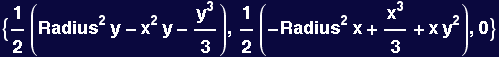
It is easy to see that this is the curl of Stooge, where

${1/2 (Radius^2 y - x^2 y - y^3/3), 1/2 (-Radius^2 x + x^3/3 + x y^2), 0}$

In fact, we could add to Stooge, any vector function that has vanishing curl--there are an infinite number of these

${0, 0, -Radius^2 + x^2 + y^2}$

Its integral doesn't care which path around the cylinder it takes, the integrand doesn't depend on P(t)

-1/2 Radius^4 Cos[t]^2 + 1/6 Radius^4 Cos[t]^4 - 1/2 Radius^4 Sin[t]^2 + Radius^4 Cos[t]^2 Sin[t]^2 + 1/6 Radius^4 Sin[t]^4

-(π Radius^4)/2

Multidimensional Integral over Irregular Domains

We will attempt to model the energy of ion just above one half of a triangular capacitor.  Suppose there is a uniformly charged surface  (σ≡charge/area=1) occupying an equilaterial triangle in the z=0 plane:
     [Graphics:HTMLFiles/Lecture-14_67.gif]
    what is the energy (voltage) of a unit positive charge located at (x,y,z)

The electrical potential goes like , therefore the potential of a unit charge located at (x,y,z) from a small surface patch at (ξ,η,0) is (σ dξ dη)/r = (dξ dη)/((x - ξ)^2 + (y - η)^2 + z^2 )^(1/2)

Therefore it remains to integrate this function over the domain η∈(0,) and ξ∈ (- ) , (-))
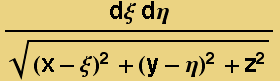∫_0^3^(1/2)/2 ∫_ (η/3^(1/2) - 1/2)^(1/2 - η/3^(1/2)) (dξ dη)/((x - ξ)^2 + (y - η)^2 + z^2 )^(1/2) dξdη

Mathematica integrates over the last iterator first:

We will try to find the potential due to a triangular patch on a particle located at (x,y,z=1)

Trying to do this directly either takes too long or there is no closed form! We have to work around it by using Indefinite Integrals

$TrianglePotentialNumeric[x_, y_, z_] := NIntegrate[1/((x - ξ)^2 + (y - η)^2 + z^2)^(1/2), {η, 0, 3^(1/2)/2}, {ξ, η/3^(1/2) - 1/2, 1/2 - η/3^(1/2) }]$

[Graphics:HTMLFiles/Lecture-14_96.gif]

The plot above is for a relatively small height z = 1/20 so the contours reveal the triangular shape of the plate at z = 0.

Now look at a somewhat larger value of z = 1/2. The plot below shows contours that are very nearly circular, indicating that the plate is behaving approximately like an equivalent point charge;

Created by Mathematica (October 18, 2005)