Solving Linear Systems, Existence and Uniqueness
Solving and Uniqueness
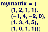
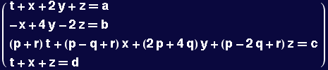
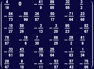
Consider the set of equations
x + 2y + z + t = a
-x + 4y - 2z = b
x + 3y + 4z + 5t = c
x + z + t = d
We illustrate how to use a matrix representation to write these out and solve them…
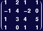
Start with the matrix of coefficients of the variables, mymatrix:
In[79]:=
![]()
Out[80]//MatrixForm=
The system of equations will only have a unique solution if the determinant of mymatrix is nonzero.
In[81]:=
Out[81]=
![]()
![]()
In[82]:=
![]()
In[83]:=
![]()
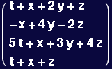
The left-hand side of the first equation will be
In[84]:=
![]()
Out[84]=
![]()
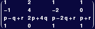
and the left-hand side of all four equations will be
In[86]:=
![]()
![]()
Out[87]//MatrixForm=
Now define an indexed variable linsys with four entries, each being one of the equations in the system of interest:
In[88]:=
![]()
In[89]:=
![]()
Out[89]=
![]()
Solving the set of equations for the unknowns ![]()
In[94]:=
![]()
Out[94]=
![]()
Doing the same thing a different way, using Mathematica's LinearSolve function:
In[95]:=
![]()
In[96]:=
Out[96]=
![]()
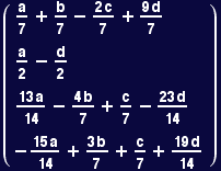
And yet another way, based on ![]() =
=![]()
![]()
![]() =
= ![]()
![]()
In[98]:=
Out[98]//MatrixForm=
When determinants are zero
Create a matrix with one row as a linear combination of the others
In[99]:=
![myzeromatrix = {mymatrix[[1]], mymatrix[[2]], p * mymatrix[[1]] + q * mymatrix[[2]] + r * mymatrix[[4]], mymatrix[[4]]} ;](HTMLFiles/Lecture-07_32.gif)
![]()
Out[100]//MatrixForm=
In[101]:=
![]()
Out[101]=
![]()
In[102]:=
![]()
![]()
Out[102]=
![]()
This was not expected to have a solution because one of four equations in the system was a linear combination of others in the system. Effectively, we were asking Mathematica to solve a system of three equations in four unknowns. The rank of a square matrix of coefficients is equal to the number of linearly independent equations in the system. The null space of the matrix will be empty when the equations are all linearly independent.
In[103]:=
Out[103]=
![]()
Out[104]=
![]()
In[109]:=
Out[109]=
![]()
Out[110]=
![]()
Try solving this inhomogeneous system of equations using Solve:
In[111]:=
![]()
Out[111]=
![]()
In[112]:=
![]()
In[114]:=
![]()
Out[114]//MatrixForm=
In[115]:=
![]()
Out[115]=
![]()
No solution, as expected, Let's see what happens if we ask Mathematica to solve the homogeneous problem:
In[118]:=
![]()
![]()
Out[118]=
![]()
In this case, Mathematica gives a relationship between the variables, but because there are fewer equations than variables, there is still no unique solution.
Determinants
In[119]:=
![]()
Start by building a routine to make vectors containing six random numbers on the interval {-1,1}:
In[120]:=
![]()
In[121]:=
![]()
Out[121]=
![]()
In[122]:=
![]()
Out[122]=
![]()
Now use rv to make a 6 x 6 matrix, then find its determinant:
In[123]:=
![]()
Out[123]=

In[124]:=
![]()
Out[124]=
![]()
Switching two rows changes the sign but not the magnitude of the determinant:
In[125]:=
Out[125]=
![]()
In[127]:=
![]()
Out[127]=
![]()
Multiply one row by a constant and calculate determinant:
![]()
![]()
Out[128]=
![]()
Multiply two rows by a constant and calculate determinant:
In[129]:=
![]()
Out[129]=
![]()
Multiply all rows by a constant and calculate determinant:
In[130]:=
![]()
Out[130]=
![]()
In[131]:=
![]()
In[132]:=
![]()
Out[132]=

Example of numerical precision: if one row of a 6 x 6 matrix is a linear combination of the other five rows, its determinant should evaluate to zero…
In[133]:=
Out[133]=
![]()
In[134]:=
Out[134]=
![]()
Showing that the determinant of a product of matrices is the product of determinants
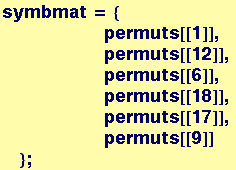
Creating a symbolic matrix
In[135]:=
![]()
In[138]:=
Out[138]=

Out[139]=
![]()
In[140]:=
![]()
Out[141]//MatrixForm=
In[150]:=
![]()
Out[150]=
![]()
Creating a matrix of rational numbers
In[143]:=
![randommat = Table[Table[Random[Integer, {-100, 100}]/Random[Integer, {-100, 100}], {i, 6}], {j, 6}] ;](HTMLFiles/Lecture-07_96.gif)
![]()
Out[144]//MatrixForm=
In[151]:=
![]()
Out[151]=
![]()
In[146]:=
![]()
Out[146]=

In[153]:=
![]()
Out[153]=
![]()
Does the determinant of a product depend on the order of multiplication?
In[154]:=
![]()
Out[154]=

In[155]:=
![]()
Out[155]=
![]()
However, the product of two matrices depends on which matrix is on the left and which is on the right
In[156]:=
![]()
Out[156]//MatrixForm=
Linear Transformations
We now demonstrate the use of matrix multiplication for manipulating an object, specifically an octohedron. The Octahedron is made up of eight polygons and the initial coordinates of the vertices were set to make a regular octahedron with its main diagonals parallel to axes x,y,z. The faces of the octahedron are colored so that rotations and other transformations can be easily tracked.
In[157]:=
In[158]:=
![]()
![[Graphics:HTMLFiles/Lecture-07_113.gif]](HTMLFiles/Lecture-07_113.gif)
Out[158]=
![]()
In[159]:=
![]()
![[Graphics:HTMLFiles/Lecture-07_116.gif]](HTMLFiles/Lecture-07_116.gif)
Out[159]=
![]()
In[160]:=
![]()
Out[160]//InputForm=
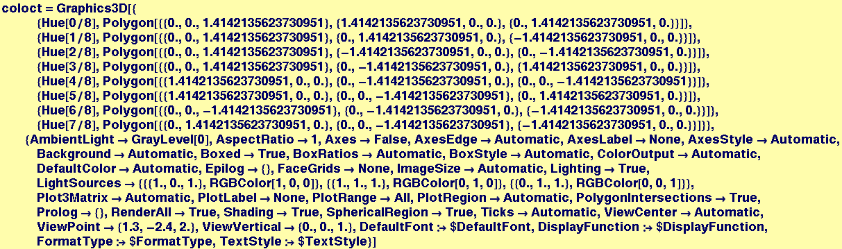
Graphics3D[{Polygon[{{0., 0., 1.4142135623730951},
{1.4142135623730951, 0., 0.}, {0., 1.4142135623730951, 0.}}],
Polygon[{{0., 0., 1.4142135623730951}, {0., 1.4142135623730951, 0.},
{-1.4142135623730951, 0., 0.}}],
Polygon[{{0., 0., 1.4142135623730951}, {-1.4142135623730951, 0., 0.},
{0., -1.4142135623730951, 0.}}],
Polygon[{{0., 0., 1.4142135623730951}, {0., -1.4142135623730951, 0.},
{1.4142135623730951, 0., 0.}}],
Polygon[{{1.4142135623730951, 0., 0.}, {0., -1.4142135623730951, 0.},
{0., 0., -1.4142135623730951}}],
Polygon[{{1.4142135623730951, 0., 0.}, {0., 0., -1.4142135623730951},
{0., 1.4142135623730951, 0.}}],
Polygon[{{0., 0., -1.4142135623730951}, {0., -1.4142135623730951, 0.},
{-1.4142135623730951, 0., 0.}}],
Polygon[{{0., 1.4142135623730951, 0.}, {0., 0., -1.4142135623730951},
{-1.4142135623730951, 0., 0.}}]}, {AmbientLight -> GrayLevel[0],
AspectRatio -> Automatic, Axes -> False, AxesEdge -> Automatic,
AxesLabel -> None, AxesStyle -> Automatic, Background -> Automatic,
Boxed -> True, BoxRatios -> Automatic, BoxStyle -> Automatic,
ColorOutput -> Automatic, DefaultColor -> Automatic,
DefaultFont :> $DefaultFont, DisplayFunction :> $DisplayFunction,
Epilog -> {}, FaceGrids -> None, FormatType :> $FormatType,
ImageSize -> Automatic, Lighting -> True,
LightSources -> {{{1., 0., 1.}, RGBColor[1, 0, 0]},
{{1., 1., 1.}, RGBColor[0, 1, 0]}, {{0., 1., 1.},
RGBColor[0, 0, 1]}}, Plot3Matrix -> Automatic, PlotLabel -> None,
PlotRange -> All, PlotRegion -> Automatic,
PolygonIntersections -> True, Prolog -> {}, RenderAll -> True,
Shading -> True, SphericalRegion -> False, TextStyle :> $TextStyle,
Ticks -> Automatic, ViewCenter -> Automatic,
ViewPoint -> {1.3, -2.4, 2.}, ViewVertical -> {0., 0., 1.}}]
The object coloct is defined below to draw an octahedron and it invokes the Polygon function to draw the triangular faces by connecting three points at specific numerical coordinates. Note that each triangles' three vertices are each specified by a vector.
In[161]:=
![]()
Out[162]=
![]()
In[163]:=
![]()
![[Graphics:HTMLFiles/Lecture-07_123.gif]](HTMLFiles/Lecture-07_123.gif)
Out[163]=
![]()
Now a matrix tmat is defined that will operate on the coordinate vectors fed to the Polygon function in coloct. In this first example, each z coordinate will be changed to -z:
In[164]:=
![]()
![]()
![]()
Out[166]//MatrixForm=
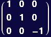
The Replace is used to modify the coordinates fed to the Polygon function in coloct by matrix multiplication of the vertex vectors:
In[167]:=
![[Graphics:HTMLFiles/Lecture-07_130.gif]](HTMLFiles/Lecture-07_130.gif)
Out[167]=
![]()
The program seetrans does the same thing by feeding a matrix tranmat to operate on the vertex vectors before Polygon is executed:
In[168]:=
![]()
When tranmat is the identity matrix, the octagon is rendered in its initial orientation.
In[169]:=
![]()
![[Graphics:HTMLFiles/Lecture-07_134.gif]](HTMLFiles/Lecture-07_134.gif)
Out[169]=
![]()
The next command rotates the octagon by 45° about the vertical (z) axis…
In[170]:=
![]()
![[Graphics:HTMLFiles/Lecture-07_137.gif]](HTMLFiles/Lecture-07_137.gif)
Out[170]=
![]()
And the next command both rotates it 180° about x and y and stretches it by a factor of 5 along z.
In[171]:=
![]()
![[Graphics:HTMLFiles/Lecture-07_140.gif]](HTMLFiles/Lecture-07_140.gif)
Out[171]=
![]()

![]()

![]()
| Created by Mathematica (September 23, 2005) |