Graphics and Plotting

Mathematica has a large number of built-in graphics programs for plotting and exploring mathematics graphically and for plotting and visualizing data.  Graphs and plots are effective ways of conveying complex information.  It is important to learn how to create and manipulate plots and graphics.  Mathematica is very rich in its graphical functions—we will explore just a small subset of all its capabilities.  We can get an idea of how many plotting routines are available byusing a wildcard:

In[116]:=

System`

Global`

Graphics`Animation`

Graphics`ContourPlot3D`

Graphics`FilledPlot`

Graphics`Graphics`

Graphics`Graphics3D`

Graphics`ImplicitPlot`

Graphics`InequalityGraphics`

Graphics`Legend`

Graphics`MultipleListPlot`

Graphics`ParametricPlot3D`

Graphics`PlotField`

Graphics`PlotField3D`

This is much less than are available in the standard packages; these will be discussed later, but here's what becomes available after loading the Graphics Packages:

In[117]:=

While Mathematica has a large number of plotting routines, no one program does everything we need.  It can be useful to export numbers and graphics from Mathematica and operate on them individually or with other specialized programs.  The number of different creative graphical solutions available grows geometrically with the number of different graphical tools that are mastered.
Here, we will just produce a number of examples of plots and graphics... (Note, I use a file "init.m" to set some options.  Your plots may look different from what we see in lecture. If you want to use my init.m you can download it from here. Where to locate your init.m file depends on the operating system you are using, check out init.m in the Master Index in the Help Browser.

Two-Dimensional Graphics

Plot, ParametricPlot, LogPlot, etc

In[119]:=

Out[119]=

In[120]:=

Out[120]=

In[121]:=

Out[121]=

In[122]:=

Out[122]=

In[123]:=

Out[123]=

In[124]:=

Out[124]=

ParametricPlot produces a 2-D graph as a function of a single parameter, e.g. t. The cartesian coordinates, e.g. x and y, are specified as functions x(t) and y(t). Thus, a continuous variation of the single parameter t will trace out a trajectory in the x-yˆplane.

In[125]:=

In[126]:=

In[127]:=

Out[127]=

In[128]:=

Out[128]=

The next statement attempts to use the Table function to produce a list of six LuckyClover functions and then make one parametric plot of all of them.

In[129]:=

Out[129]=

It is necessary to use the Evaluate command to get this to work.

In[130]:=

In[131]:=

Out[131]=

In[132]:=

Out[132]=

In[133]:=

In[134]:=

Out[134]=

Out[135]=

Out[136]=

In[137]:=

In[138]:=

In[139]:=

Out[139]=

In[140]:=

Out[140]=

In[141]:=

Out[141]=

In[142]:=

Out[142]=

In[143]:=

In[144]:=

Out[144]=

In[145]:=

In[146]:=

Out[146]=

Plotting Data

ListPlot, PieChart, Histogram, Barchart, etc

In[147]:=

In[148]:=

Out[148]=

In[149]:=

Out[149]=

In[150]:=

Out[150]=

The next plot illustrates the variation of melting temperature as a function of atomic number…

In[151]:=

Out[151]=

In[152]:=

Out[152]=

In[153]:=

Out[153]=

The next line matches up values of density with melting temperature…

In[154]:=

Out[154]=

In[155]:=

Out[155]=

In[156]:=

Out[156]=

Three-Dimensional Graphics

Plot3D, ContourPlot, DensityPlot, etc

In[157]:=

In[158]:=

SheetOLatticeCharge represents the electric field produced by an 11 by 11 array of point charges arranged on the x-y plane at z = 0. The following command evaluates and plots the field variation in the plane z = 0.25:

In[159]:=

Out[159]=

Note below how theplot is set to contain the output of the Plot3D command.

In[160]:=

Out[160]=

Now we can adjust the viewpoint of theplot, without recalculating the entire plot, using the Show command:

In[161]:=

In[162]:=

In[163]:=

Out[163]=

In[164]:=

Out[164]=

In[165]:=

Out[165]=

In[166]:=

Out[166]=

In[167]:=

Out[167]=

Graphics Primitives

It can be useful to be able to build up arbitrary graphics objects piece-by-piece using simple "graphics primitives" like Circle:

In[168]:=

Out[168]=

In[169]:=

Out[169]=

In[170]:=

Out[170]=

Now we take a simple plot…

In[171]:=

Out[171]=

and overlay some text in places of our own choosing…

In[172]:=

Out[172]=

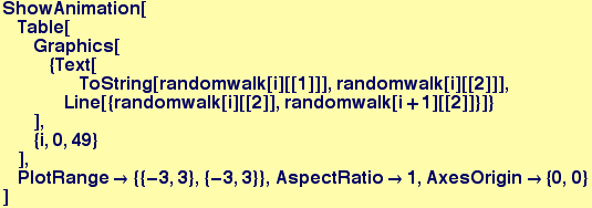
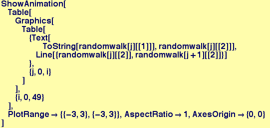
Many processes in the natural world can be modelled by random walks. An example is the trajectory of a particular  molecule in a gas at low pressure.  The next few lines of code produce random walks and display them graphically:

In[173]:=

Out[173]=

In[174]:=

Out[174]=

In[175]:=

In[176]:=

Out[176]=

In[177]:=

Out[177]=

In[178]:=

Out[178]=

In[179]:=

In[180]:=

In[181]:=

In[182]:=

Out[182]=

These last two plots have to do with the orientation dependence of the surface energy of a 2-D crystal (GammaPlot)and the equilibrium shape that a single crystal having this surface energy will adopt to minimize its total surface energy.

In[183]:=

In[184]:=

Out[184]=

In[185]:=

Out[185]=

The inner envelope of the tangent lines to the GammaPlot in the figure above illustrates the energy-minimizing shape of the crystal. For this particular GammaPlot, the shape is approximately a square but the corners are rounded.

Created by Mathematica  (September 15, 2005)